DATA STORIES | GEOSPATIAL ANALYTICS | KNIME ANALYTICS PLATFORM

Discovering Andalucía with KNIME: Montoro and Barbate

Join me on this geospatial adventure to two of my favourite places to live and vacation in the beautiful region of Andalucía, Spain

Part 1: Discovering Montoro and Barbate

Our journey begins with a detailed exploration of Montoro and Barbate. To do this, we create a workflow that will help us describe and visualize these two charming places and nearby points of interest.

Step 1: Input location names

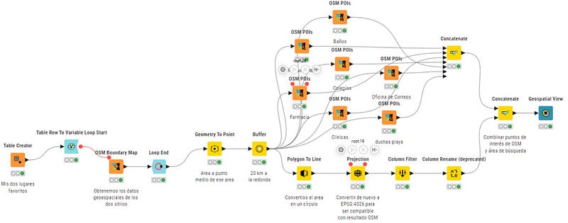
In the first step, we use the Table Creator node to input the names of our two favourite places: Montoro to live and Barbate to vacation.

Step 2: Get geospatial data with the OSM Boundary Map node

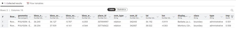
Now that we have the names of our places, it’s time to obtain their geospatial data. We use the OSM Boundary Map node to extract this information for Montoro and Barbate. This node allows us to get polygons representing the geographic areas of interest.

Step 3: From areas to midpoints

In the next step, we use the Geometry to Point node to convert these polygons into midpoints. This allows us to represent each place with a single point on the map, which will be useful later.

Step 4: Draw circular areas

To better visualize the surrounding areas of our favourite places, we use the Buffer node. This node creates asymmetric circular areas around the midpoints we generated in the previous step. In our case, we create a circle with a 20 km radius around each location, which is why we transformed polygons into midpoints in the previous step.

Note. The output of a the Buffer node is again a polygon, representing the circular areas.

Step 5: Retrieve points of interest within circular area

Within the circular areas we want to identify a variety of points of interest. We use the OSM POIs node to obtain geospatial data for places like restaurants, schools, post offices, beach showers, etc.

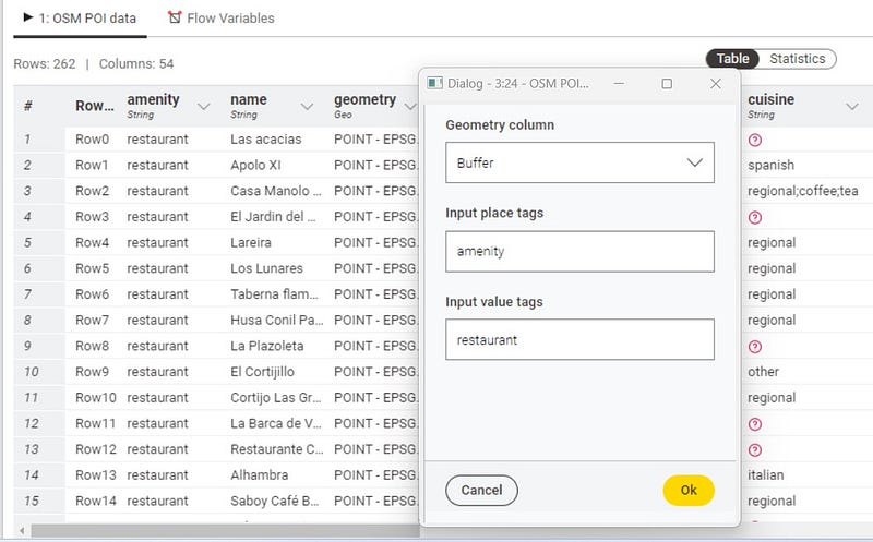
This node is quite interesting as it provides us with a lot of information. For example, for restaurants, we could select a restaurant based on its type of cuisine or opening hours.

We also use the Polygon to Line node to transform the circular areas into circular lines, and with the Projection node, we convert the data to be compatible with the CRS of the data obtained from the OSM POIs node. Finally, we use the Concatenate node to merge these two datasets.

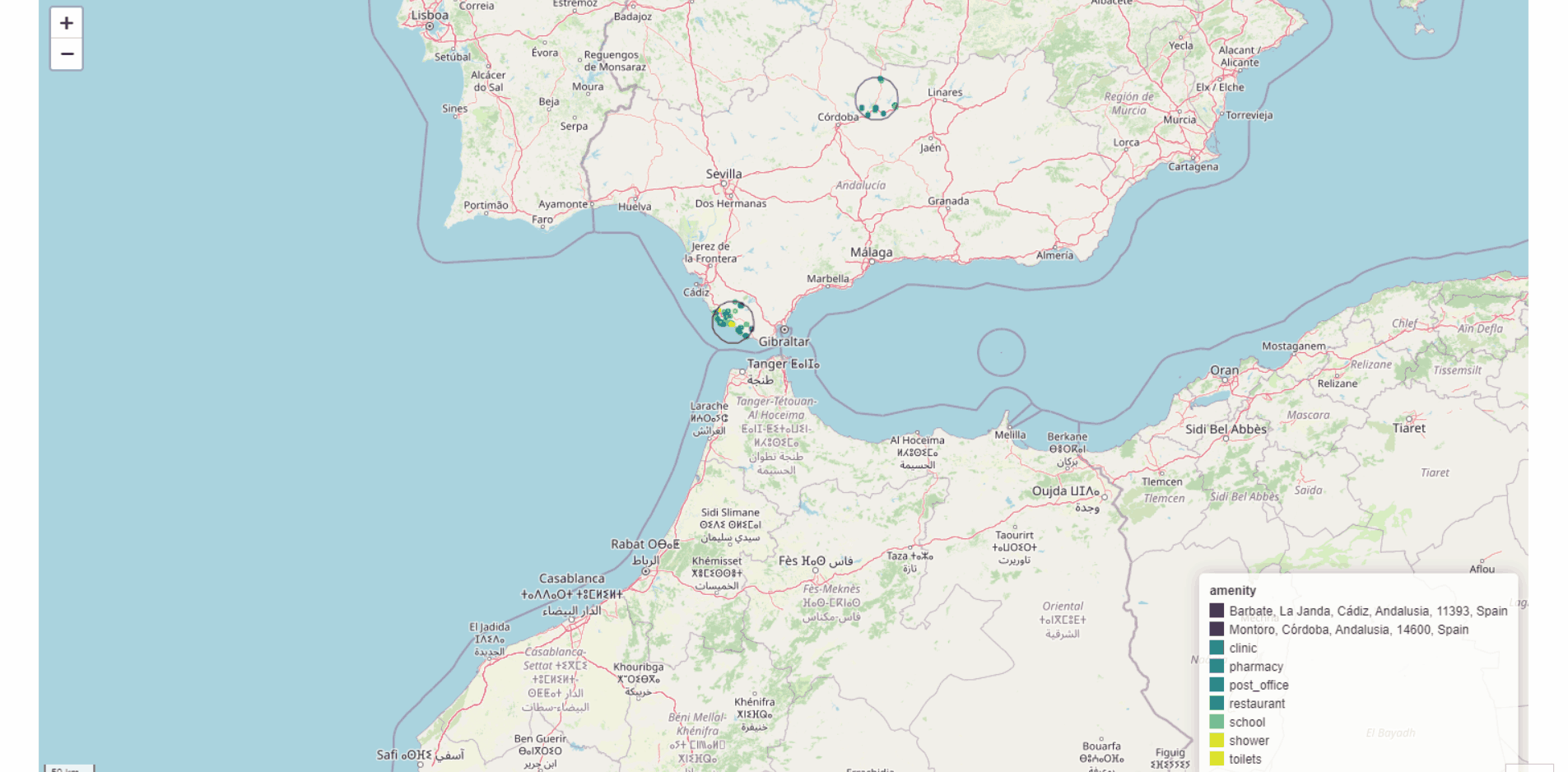
Step 6: Visualize with the Geospatial View node

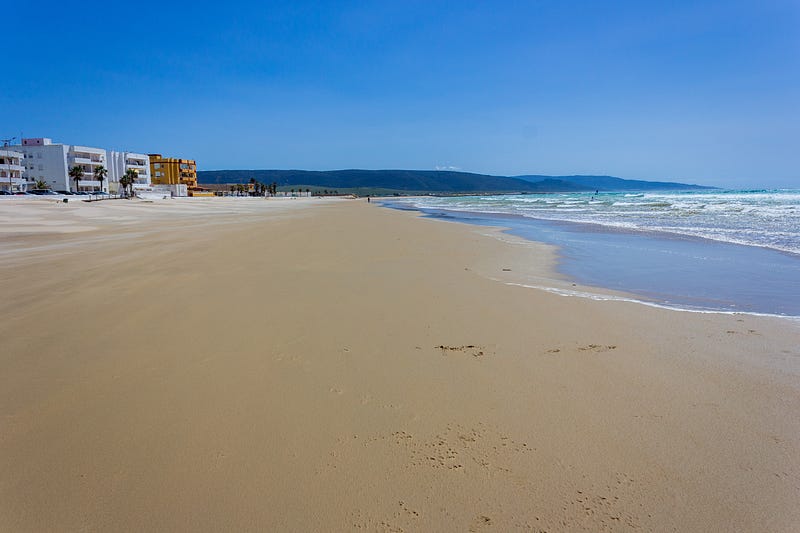
It’s time to see the results of our work. We use the Geospatial View node to visualize all the information collected so far. We can see Montoro and Barbate, each with its 20 km radius circle, and the points of interest we’ve found.

Part 2: Exploring the route from Montoro to Barbate

Our geospatial journey wouldn’t be complete without exploring the car journey from Montoro to Barbate. For this, we’ve created another workflow.

Step 1: Get geospatial data of Andalucía

First, we enter the name “Andalucía” in the Table Creator node and use the OSM Boundary Map node to obtain the geospatial data for this region, just like we did for Montoro and Barbate.

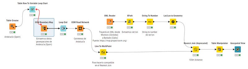
Step 2: Extract road network data

The magic begins with the OSM Road Network node, which extracts all the road network data in Andalucía. We then transform the linestrings contained in the geometry columns to a series of points representing the route data using the Line to Multipoint node.

Step 3: Get route data from Montoro to Barbate

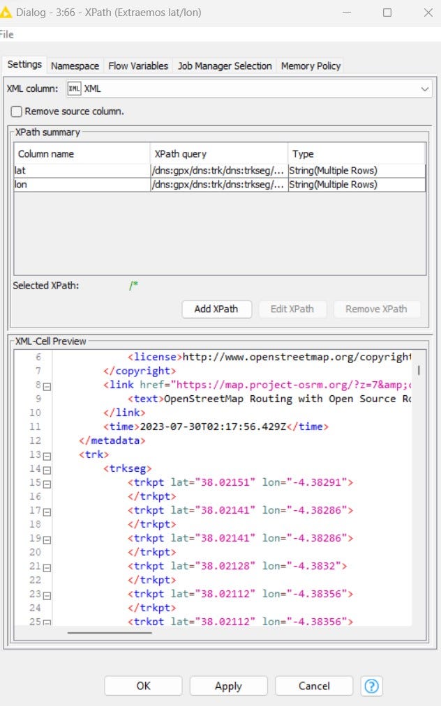
To obtain the geospatial data for the route from Montoro to Barbate, we use the website https://map.project-osrm.org/ and obtain data in XML format. Then, we use the XML Reader node and extract the latitude and longitude data with the XPath node. These data are then converted to geometry with the Lat/Lon to Geometry node.

Step 4: Merging the data

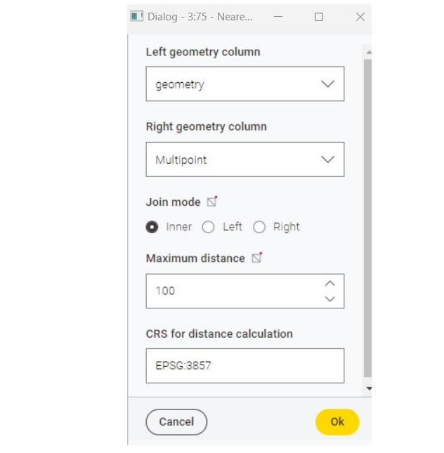
The Nearest Join node is a wonderful tool that allows us to join the geospatial data of roads with the route obtained earlier, as long as the points are at a max distance of 100 meters (user-defined distance). Finally, we clean the table with the Table Manipulator node to get a clear and concise visualization.

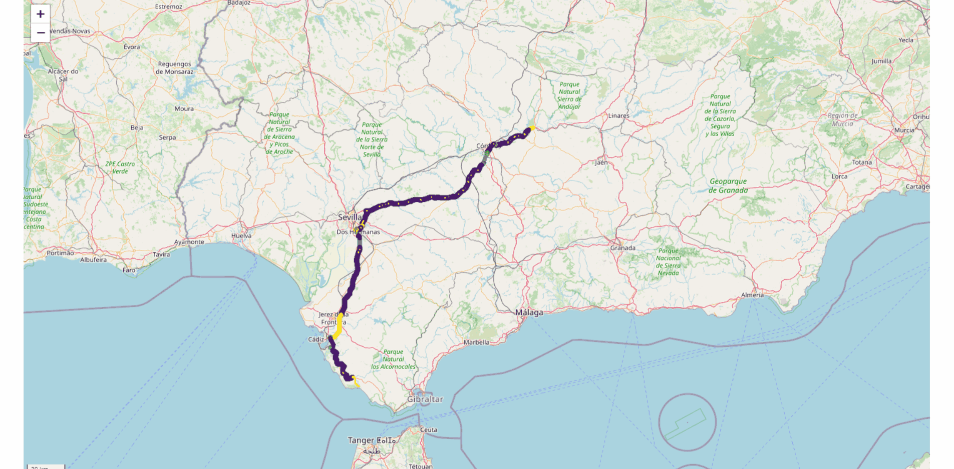
Step 5: Visualize the route

Now we can visualize the route from Montoro to Barbate! With this visualization, we can identify whether we’re travelling on highways or secondary roads, know the maximum speed, and much more. We can even change the line or colour based on the speed or type of road!

Conclusion

KNIME’s ability to manipulate and visualize geospatial data has made this experience exciting and enriching. I hope you’ve enjoyed this journey with me and that it has inspired you to explore your favourite places using KNIME Analytics Platform.

If you want to stay updated on more of my geospatial adventures and data science insights, make sure to follow me on LinkedIn and Twitter and subscribe to my weekly KNIME newsletter in Spanish on LinkedIn.

Thank you for joining me on this geospatial adventure!

Until the next exploration, happy data wrangling with KNIME!