Dimensionality reduction with PCA and t-SNE in Python

Data Science Society Workshop 18: What is dimensionality reduction, PCA implementation, t-SNE implementation

This year, as the Head of Science for the UCL Data Science Society, the society is presenting a series of 18 workshops covering topics such as introduction to Python, a Data Scientists toolkit, and Machine learning methods throughout the academic year. For each of these the aim is to create a series of small blog posts that will outline the main points with links to the full workshop for anyone who wishes to follow along. All of these can be found in our GitHub repository and will be updated throughout the year with new workshops and challenges.

The eighteenth workshop in the series, as part of the Data Science with Python workshop series, covers Dimensionality Reduction methods. In this workshop, we cover what is dimensionality reduction along with the implementation of Principal Component Analysis and t-Distributed Stochastic Neighbor Embedding methods. As always, this blog post is a summary of the complete workshop which can be found here which also covers data preparation and feature extraction using Random Forest Classification.

If you missed any of our last three workshops you can find these here

What is dimensionality reduction?

Dimensionality reduction comes (in most cases) under the heading of unsupervised machine learning algorithms meaning that we don’t have a specific target to aim for. The main aim of this method is to either reduce the number of features in a dataset, so as to reduce the resources required for the model, or to aid in visualising the data before any analysis is performed. This is done by reducing the number of attributes or variables in the dataset while attempting to keep as much of the variation in the original dataset as possible. This is a preprocessing step meaning that it is mostly performed before we create or train any model which separates it from feature extraction which is usually done after the initial modeling.

There are many algorithms that can be used for dimensionality reduction but they are primarily drawn from two main groups of linear algebra and manifold learning:

Linear algebra

This draws from matrix factorisation methods which can be used for dimensionality reduction by examining the linear relationship between variables that we may be using. Common methods within this branch include:

• Principal Components Analysis
• Singular Value Decomposition
• Non-Negative Matrix Factorisation
• Factor Analysis
• Linear Discriminant Analysis

Manifold learning

This differs from linear algebra methods in that this uses non-linear approaches to dimensionality reduction and as such can often capture more complex relationships between variables than linear algebra methods can. Some of the popular methods within this branch include:

• Isomap embedding
• Locally Linear Embedding
• Multidimensional scaling
• Spectral embedding
• t-distributed Stochastic Neighbor Embedding

Feature extraction

This group of methods may loosely fall under the umbrella of dimensionality reduction as while the methods above create new combinations of variables from existing variables, feature extraction simply removes features. We have already seen this with Feature importance from Random Forests, but popular methods in this regard include:

• Backward Elimination
• Forward Selection
• Random Forests

Each algorithm under the Dimensionality reduction umbrella offers a different approach to the challenge of reducing the number of dimensions. This often means that there is no best dimensionality reduction that can be used in all cases. It also means there is no easy way to find the best algorithm for your data without using controlled experiments and broad exploration. To this extent, we will cover an implementation of PCA and t-SNE on the NBA dataset with the aim of visualising the data in two dimensions in regards to a player's position.

PCA

PCA is just one of the linear algebra methods of dimensionality reduction. This helps us in extracting a new set of variables from an existing large set of variables, with these new variables taking the form of Principal Components. The aim of this is to capture as much information as possible in the smallest amount of principal components. The fewer the variables obtained while minimising the loss of information helps with model training in terms of the computing resources and time and helps with visualisation.

Within this, a principal component is a linear combination of variables and is organised in a way that the first principle component explains the maximum amount of variance in the dataset. The second principal component then tries to explain the remaining variance in the dataset while being uncorrelated with the first and so on.

To implement a PCA algorithm we need to normalise the data because otherwise it will lead to a large focus on variables with large variance which is undesirable. This means that we should not apply PCA to categorical variables as although we can turn them into numerical variables they will only take on values of 0 and 1 which will naturally be high in variance.

For this, we will use the StandardScaler from the scikit-learn library to scale the data before we implement the model:

#import the standard scaler
from sklearn.preprocessing import StandardScaler

#initialise the standard scaler
sc = StandardScaler()

#create a copy of the original dataset
X_rs = X.copy()

#fit transform all of our data
for c in X_rs.columns:
    X_rs[c] = sc.fit_transform(X_rs[c].values.reshape(-1,1))

Where we can then implement the model on the normalised data as follows:

#import the PCA algorithm from sklearn
from sklearn.decomposition import PCA

#run it with 15 components
pca = PCA(n_components=15, whiten=True)

#fit it to our data
pca.fit(X_rs)

#extract the explained variance
explained_variance = pca.explained_variance_ratio_
singular_values = pca.singular_values_

Now that we have fit the PCA to our data, we actually need to evaluate the components it creates. We can do this through the explained variance ratio which can be used to see how useful the principal components can be and hence selecting ones to be used in the model. We can visualise this as:

#create an x for each component
x = np.arange(1,len(explained_variance)+1)

#plot the results
plt.plot(x, explained_variance)

#add a y label
plt.ylabel('Share of Variance Explained')
plt.title("PCA explained variance plot")
plt.xlabel("Components")

#show the resuling plot
plt.show()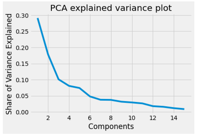

#iterate over the components
#to print the explained variance
for i in range(0, 15):
    print(f"Component {i:>2} accounts for {explained_variance[i]*100:>2.2f}% of variance")

If we were to use this data in a model then we would want to decide how many components to use in our model to balance the trade-off between computing resources and model performance. For this, there are a couple of methods we can use to choose the optimal number of principal components:

• Examining the knee in the explained variance plot, which in our case appears around 4- 6 Principles Components
• Keeping components that account for more than 1% of the variance in the dataset, which in our case will be after 14 Components
• Keeping variables that add up to 80% of explained variance in the model, which in our case would be the first 7 Components.

This can depend on the purpose of the principal component analysis and what model you are implementing. In our case, we want to try to visualise the data in two dimensions and how that relates to our target variable. Thus we can implement this as:

#set the components to 2
pca = PCA(n_components=2, whiten=True) 
#fit the model to our data and extract the results
X_pca = pca.fit_transform(X_rs)

#create a dataframe from the dataset
df = pd.DataFrame(data = X_pca,
                 columns = ["Component 1", 
                            "Component 2"])

#merge this with the NBA data
NBA = pd.merge(NBA,
              df,
              left_index=True,
              right_index=True,
              how = "inner")

#plot the resulting data from two dimensions
g = sns.jointplot(data = NBA,
                 x = "Component 1",
                 y = "Component 2",
                 hue = "Pos")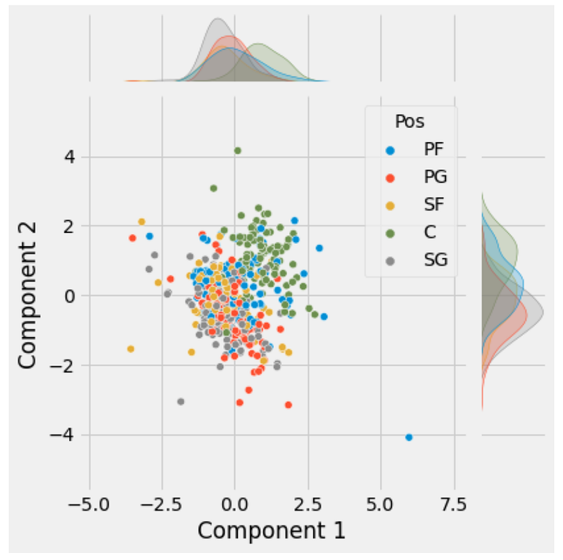

What we can see from this plot is that reducing the data to two components hasn’t necessarily shown a clear relationship between the players' position and their statistics. What we may be able to extract from this is that the Centre position may be unique from the rest of the positions, with a few merging with the Power Forward Position. While at the same time there is quite a mixture between the Point Guard, Shooting Guard and Small Forward which is to be expected to some degree.

Of course, whether you want this in two principal components or more (14 components had a variance of greater than 1%) will depend on what you want to ultimately do with the data. In the case of the earlier Random Forest Classifier workshop, we may want to use 14 components in the model rather than the 23 we originally started with given the rest may be noise and just increase model complexity.

t-SNE

t-SNE is another dimensionality reduction algorithm but unlike PCA is able to account for non-linear relationships. In this sense, data points can be mapped in lower dimensions in two main ways:

• Local approaches: mapping nearby points on the higher dimensions to nearby points in the lower dimension also
• Global approaches: attempting to preserve the geometry at all scales so keeping nearby points close together while keeping far away points away from each other as well

t-SNE is one of the few dimensionality reduction algorithms that is able to retain both structure in the lower dimension data by calculating the probability similarity of points in high and low dimensional space.

The outputs of t-SNE are often referred to as dimensions that are created with the data where the inherent features are no longer identifiable in the data. This means we cannot make any direct inference based only on the output of t-SNE, restricting this to mostly data exploration and visualisation, although the outputs can also be used in classification and clustering (although not with a test and train dataset).

When implementing a t-SNE algorithm there are a few key parameters that we need to pay attention to:

• n_components : The dimensions to be created from the data
• perplexity : related to the number of nearest neighbors used in other manifold learning algorithms it is used to determine the trade-off between global and local relationships in the model to be retained. While it is noted t-SNE is often not very sensitive to this parameter it should be smaller than the number of points with the optimal range suggested to be within 5 and 50
• learning_rate : The learning rate can often be a critical parameter to how the model behaves so it can be worth exploring the parameter space in this regard, but it is often between 100 and 1000.

The scikit-learn documentation recommends that we use PCA or truncated SVD before t-SNE if the number of features in the dataset is more than 50 because of the complexity of the algorithm. However, in our case, this shouldn’t be an issue so we can implement the model on the data that we have already. Since our aim is mainly visualisation then we can set the number of dimensions to two to be able to plot on a 2D visualisation as below:

#import the method
from sklearn.manifold import TSNE

#set the hyperparmateres
keep_dims = 2
lrn_rate = 700
prp = 40

#extract the data as a cop
tsnedf = X_rs.copy()

#creae the model
tsne = TSNE(n_components = keep_dims, 
            perplexity = prp, 
            random_state = 42,
            n_iter = 5000,
            n_jobs = -1)

#apply it to the data
X_dimensions = tsne.fit_transform(tsnedf)
#check the shape
X_dimensions.shape

#out:
(530, 2)

Which we can then visualise this as:

#create a dataframe from the dataset
tsnedf_res = pd.DataFrame(data = X_dimensions,
                         columns = ["Dimension 1", 
                                "Dimension 2"])

#merge this with the NBA data
NBA = pd.merge(NBA,
              tsnedf_res,
              left_index=True,
              right_index=True,
              how = "inner")

#plot the result
g = sns.jointplot(data = NBA,
                 x = "Dimension 1",
                 y = "Dimension 2",
                 hue = "Pos")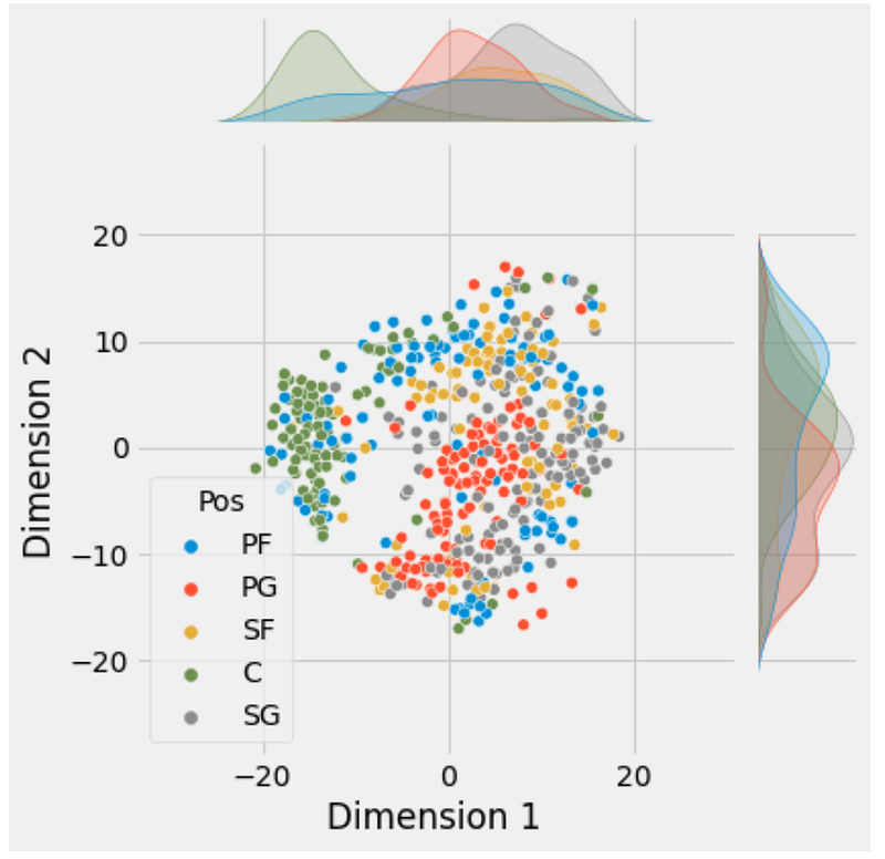

What we can see here is that we get a slightly clearer picture of the different positions to some degree than we did with PCA before. We can see now that the Centre position appears more distinct, the Shooting Guard appears very widely distributed, while the Point Guards tend to concentrate together, along with the Small and Power Forward appearing together.

This makes it slightly clearer and suggests that the relationship between variables may indeed be non-linear and so t-SNE may be better on this dataset. Of course, in thinking about this you have to be mindful of what you want to use the Dimensions or Principle Components for.

If you want any further information on our society feel free to follow us on our socials:

Facebook: https://www.facebook.com/ucldata

Instagram: https://www.instagram.com/ucl.datasci/

LinkedIn: https://www.linkedin.com/company/ucldata/

And if you want to keep up to date with stores from the UCL Data Science Society and other amazing authors, feel free to sign up to medium using my referral code below.

Or view some of my other articles on Medium