
Digging Deeper: Exploring Extended Common Neighbors in Link Prediction
Link prediction is a prominent area of research in complex network analysis, with applications in various fields including network evolution analysis, recommendation systems, and protein interaction analysis in biological networks. The main objective of link prediction is to estimate missing or hidden links between disconnected nodes in a network. Over the years, numerous algorithms and models have been developed for link prediction, categorized into similarity-based approaches and learning-based approaches.
Similarity-based approaches calculate similarity scores between unconnected nodes based on available information. The underlying hypothesis is that nodes with higher similarity are more likely to have a link between them. This idea is straightforward and widely explored, making similarity-based approaches the mainstream in link prediction research. The Common Neighbors (CN) index, for instance, simply counts the number of common neighbors between two nodes. The Adamic-Adar (AA) and Resource Allocation (RA) indexes, variations of the CN index, adjust for the influence of highly connected common neighbors. These indexes are considered local methods as they rely on local structural information.
In addition to local methods, global and quasi local methods have been proposed by researchers, such as Katz, SimRank, Random Walks with Restart, Local Path, FriendLink, and Local Random Walk. However, as complex networks continue to grow in size, local methods remain favorable due to their efficiency in terms of running time. Consequently, this study focuses on local methods.
Cannistraci et al. introduced the CAR index, which suggests that links between common neighbors, referred to as local-community-links (LCLs), hold more significance in link prediction than individual common neighbors. The CAR index proposes that the likelihood of two nodes being connected is higher if their common first neighbors belong to a tightly interconnected group known as a local community (LC). The internal links within the LC are referred to as local community links (LCLs), as shown in Figure 1.
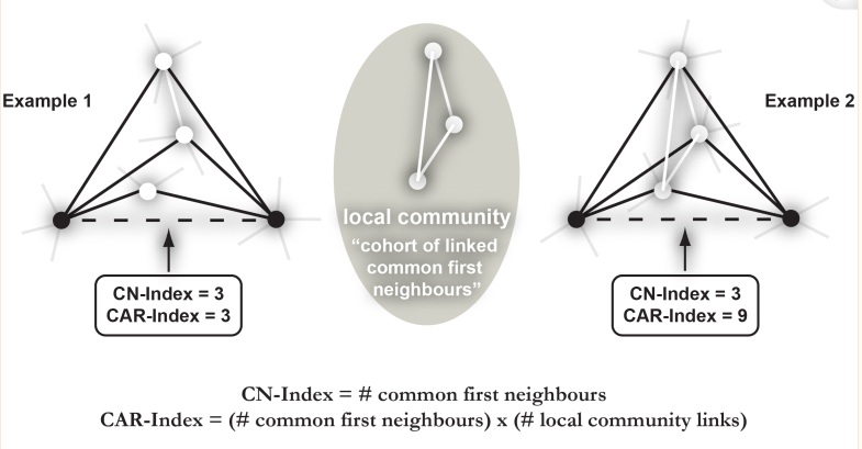
When a link or node directly interacts with a seed node, it belongs to the first-level neighborhood and provides first-level topological information. On the other hand, a link or node that interacts with the first-level neighborhood conveys second-level information. Second-level information is valuable and can significantly enhance topological link prediction. However, it is also noisy, making it challenging to integrate with the first-level information.
CAR is designed to capture and filter meaningful second-level information by leveraging common first neighbors. The internal links between common first neighbors carry valuable second-level information. As these common first neighbors interact more frequently, they form a local community that encompasses the two seed nodes. Consequently, the likelihood of a candidate link between the seed nodes increases.
The code to compute this CAR index is shown below
import networkx as nx
import pandas as pd
import numpy as np

def compute_local_community_links(G, i, j):
    # The common neighbourhood of the nodes i and j
    common_neighbors = list(nx.common_neighbors(G, i, j))

    # Count the links between the common neighbors
    local_community_links = sum(1 for x in common_neighbors for y in common_neighbors if G.has_edge(x, y))

    # Divide by 2 to avoid double-counting
    local_community_links /= 2

    return local_community_links

def compute_scores(G):
    nodes = list(G.nodes)
    n = len(nodes)
    scores = []

    for i in range(n):
        for j in range(i+1, n):
            # Only compute the score if nodes i and j are not connected
            if not G.has_edge(nodes[i], nodes[j]):
                common_neighbors = len(list(nx.common_neighbors(G, nodes[i], nodes[j])))
                local_community_links = compute_local_community_links(G, nodes[i], nodes[j])
                score = common_neighbors * local_community_links
                scores.append((nodes[i], nodes[j], score))

    # Create a DataFrame of the scores
    df_scores = pd.DataFrame(scores, columns=['Node1', 'Node2', 'Score'])
    df = df_scores.sort_values(by='Score', ascending=False)

    return df

G = nx.gnp_random_graph(20, 0.4)
df_scores = compute_scores(G)
print(df_scores)
One can use this and compute similarity between nodes and associate links.
We can go deep to extend it to common neighbors of common neighbors, by going one more level deep. While selecting level-2 common neighbors of common neighbors there exist some possibilities that level-2 common neighbors are also treated as level-1 common neighbors , as shown in Figure 2. In such cases, level-2 common neighbors are extended to next level in the network and continue until further identification of level-2 common neighbors as level-1 common neighbors.
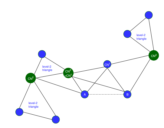
What I mean is, In Figure 2 graph, ‘A’ and ‘B’ are the nodes of interest and are colored blue. The nodes that are directly connected to either ‘A’ or ‘B’ are level-1 common neighbors . The nodes that are connected to the level-1 common neighbors(CN1) (but not directly to ‘A’ or ‘B’) are level-2 common neighbors(CN2) and are colored green.
We will create a function to get the neighbors of the neighbors and calculate the local community links and scores accordingly.
import networkx as nx
import pandas as pd
import numpy as np

def extend_common_neighbors(G, common_neighbors):

    """Extend common neighbors to next level if they are also in the current level"""
    next_level_common_neighbors = set().union(*[list(nx.neighbors(G, n)) for n in common_neighbors])
    next_level_common_neighbors.difference_update(common_neighbors)  # remove current level neighbors

    # If next level neighbors are in the current level, extend further
    while len(next_level_common_neighbors.intersection(common_neighbors)) > 0:
        common_neighbors.update(next_level_common_neighbors)
        next_level_common_neighbors = set().union(*[list(nx.neighbors(G, n)) for n in common_neighbors])
        next_level_common_neighbors.difference_update(common_neighbors)

    return next_level_common_neighbors

def compute_local_community_links_extended(G, i, j):

    """Compute local community links considering extended common neighbors"""
    common_neighbors = list(nx.common_neighbors(G, i, j))
    common_neighbors = extend_common_neighbors(G, set(common_neighbors))

    # Count the links between the common neighbors
    local_community_links = sum(1 for x in common_neighbors for y in common_neighbors if G.has_edge(x, y))

    # Divide by 2 to avoid double-counting
    local_community_links /= 2

    return local_community_links

def compute_scores_extended(G):

    """Compute link prediction scores considering extended common neighbors"""
    nodes = list(G.nodes)
    n = len(nodes)
    scores = []

    for i in range(n):
        for j in range(i+1, n):
            # Only compute the score if nodes i and j are not connected
            if not G.has_edge(nodes[i], nodes[j]):
                common_neighbors = len(list(nx.common_neighbors(G, nodes[i], nodes[j])))
                local_community_links = compute_local_community_links_extended(G, nodes[i], nodes[j])
                score = common_neighbors * local_community_links
                scores.append((nodes[i], nodes[j], score))

    # Create a DataFrame of the scores
    df_scores = pd.DataFrame(scores, columns=['NodeA', 'NodeB', 'Score'])

    df = df_scores.sort_values(by='Score', ascending=False)

    return df

G = nx.gnp_random_graph(20, 0.2)
df_scores = compute_scores_extended(G)
print(df_scores)
For each node in common_neighbors, get its neighbors in the graph G. This is done by calling nx.neighbors(G, n) for each node n in common_neighbors. The set().union(*[list(nx.neighbors(G, n)) for n in common_neighbors]) line unions all these neighbors together into a single set next_level_common_neighbors.
This function is a part of a bigger process for predicting links in a network, specifically in situations where the direct neighbors (level-1) are not providing sufficient information and you want to consider the neighbors of neighbors (level-2, level-3, and so on). By extending the neighborhood levels, you can capture more complex relationships in the network and potentially improve the accuracy of your link prediction.
Conclusion
The method of calculating node similarity based on common neighbors, and extending it to higher levels (i.e., level-2 or level-3 common neighbors), is a powerful technique for link prediction in networks. This technique can be especially useful in applications such as social network analysis, recommendation systems, bioinformatics (e.g., predicting protein-protein interactions), and any other domain where the structure of the network can be used to predict missing or future connections.
In heterogeneous network, nodes and edges can have different types, adding another layer of complexity to the task of computing similarity. The common neighbors approach can still be used, but the interpretation of what constitutes a “neighbor” and what constitutes a “connection” may differ depending on the types of nodes and edges involved. Furthermore, the importance or weight of different types of connections may vary, and this needs to be taken into account when calculating similarity scores. , While calculating node similarity based on common neighbors and their connections is a powerful technique for link prediction, it also comes with challenges in terms of computational complexity and the complexity of interpreting results in heterogeneous networks. Nonetheless, with careful implementation and interpretation, it can provide valuable insights in a wide range of applications.


