Getting Started

Did you know this in Spark SQL?

8 non-obvious features in Spark SQL that are worth knowing.

The DataFrame API of Spark SQL is user friendly because it allows expressing even quite complex transformations in high-level terms. It is quite rich and mature especially now in Spark 3.0. There are however some situations in which you might find its behavior unexpected or at least not very intuitive. This might get frustrating especially if you find out that your production pipeline produced results that you didn’t expect.

In this article, we will go over some features of Spark which are not so obvious at first sight, and by knowing them you can avoid silly mistakes. In some examples, we will also see nice optimization tricks that can become handy depending on your transformations. For the code examples, we will use Python API in Spark 3.0.

1. What is the difference between array_sort and sort_array?

Both of these two functions can be used for sorting the arrays, however, there is a difference in usage and null handling. While array_sort can only sort your data in ascending order, the sort_array takes a second argument in which you can specify whether your data should be sorted in descending or ascending order. The array_sort will place null elements at the end of the array which will also sort_array do when sorting in descending order. But when using sort_array in ascending (default) order the null elements will be placed at the beginning.

l = [(1, [2, None, 3, 1])]

df = spark.createDataFrame(l, ['id', 'my_arr'])

(
    df
    .withColumn('my_arr_v2', array_sort('my_arr'))
    .withColumn('my_arr_v3', sort_array('my_arr'))
    .withColumn('my_arr_v4', sort_array('my_arr', asc=False))
    .withColumn('my_arr_v5', reverse(array_sort('my_arr')))
).show()

+---+----------+----------+-----------+----------+-----------+
| id|    my_arr| my_arr_v2|  my_arr_v3| my_arr_v4|  my_arr_v5|
+---+----------+----------+-----------+----------+-----------+
|  1|[2,, 3, 1]|[1, 2, 3,]|[, 1, 2, 3]|[3, 2, 1,]|[, 3, 2, 1]|
+---+----------+----------+-----------+----------+-----------+

And there is one more option on how to use the function array_sort, namely directly in SQL (or as a SQL expression as argument of the expr() function) where it takes a second argument which is a comparator function (supported since Spark 3.0). With this function, you can define how the elements should be compared to create the order. This actually brings quite powerful flexibility by which you can for example sort an array of structs and define by which struct field it should be sorted. Le’ts see this example where we sort explicitly by the second struct field:

schema = StructType([
    StructField('arr', ArrayType(StructType([
        StructField('f1', LongType()), 
        StructField('f2', StringType())
    ])))
])
l = [(1, [(4, 'b'), (1, 'c'), (2, 'a')])]
df = spark.createDataFrame(l, schema=schema)

(
    df
    .withColumn('arr_v1', array_sort('arr'))
    .withColumn('arr_v2', expr(
        "array_sort(arr, (left, right) -> case when left.f2 < right.f2 then -1 when left.f2 > right.f2 then 1 else 0 end)"))
).show(truncate=False)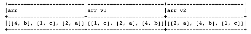

Here you can see that the comparison function expressed in SQL takes two arguments left and right which are elements of the array and it defines how they should be compared (namely according to the second field f2).

2. concat function is null-intolerant

The concat function can be used for concatenating strings, but also for joining arrays. The less obvious thing is that the function is null-intolerant, which means that if any argument is null, then also the output becomes null. So for example when joining two arrays, we can easily lose the data from one array if the other one is null unless we handle it explicitly, for instance, by using coalesce:

from pyspark.sql.types import *
from pyspark.sql.functions import concat, coalesce, array

schema = StructType([
    StructField('id', LongType()),
    StructField('arr_1', ArrayType(StringType())),
    StructField('arr_2', ArrayType(StringType()))
])

l = [(1, ['a', 'b', 'c'], None)]
df = spark.createDataFrame(l, schema=schema)

(
    df
    .withColumn('combined_v1', concat('arr_1', 'arr_2'))
    .withColumn('combined_v2', concat(coalesce('arr_1'), array(), coalesce('arr_2', array())))
).show()

+---+---------+-----+-----------+-----------+
| id|    arr_1|arr_2|combined_v1|combined_v2|
+---+---------+-----+-----------+-----------+
|  1|[a, b, c]| null|       null|  [a, b, c]|
+---+---------+-----+-----------+-----------+

3. collect_list is not a deterministic function

Aggregation function collect_list which can be used to create an array of elements after grouping by some key is not deterministic because the order of elements in the resulting array depends on the order of rows which may not be deterministic after the shuffle.

It is also good to know that non-deterministic functions are treated with special care by the optimizer, for example, the optimizer will not push filters through it as you can see in the following query:

(
  df.groupBy('user_id')
  .agg(collect_list('question_id'))
  .filter(col('user_id').isNotNull())
).explain()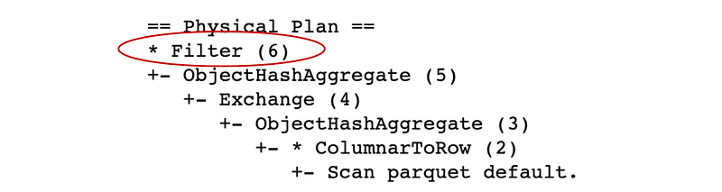

As you can see from the plan, the Filter is the last transformation, so Spark will first compute the aggregation and after that, it will filter out some groups (here we filter out group where user_id is null). It would be however more efficient if the data was first reduced by the filter and then aggregated which will indeed happen with deterministic functions such as count:

(
  df.groupBy('user_id')
  .agg(count('*'))
  .filter(col('user_id').isNotNull())
).explain()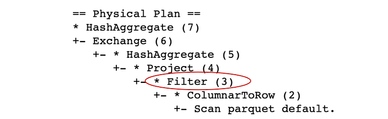

Here the Filter was pushed closer to the source because the aggregation function count is deterministic.

Besides collect_list, there are also other non-deterministic functions, for example, collect_set, first, last, input_file_name, spark_partition_id, or rand to name some.

4. Sorting the window will change the frame

There is a variety of aggregation and analytical functions that can be called over a so-called window defined as follows:

w = Window().partitionBy(key)

This window can be also sorted by calling orderBy(key) and a frame can be specified by rowsBetween or rangeBetween. This frame determines over which rows will the function be called inside the window. Some functions require also to sort the window (for example row_count) but for some functions the sort is optional. The point is that the sort can change the frame which might not be intuitive. Consider the example with sum function:

from pyspark.sql import Window
from pyspark.sql.functions import sum

l = [
  (1, 10, '2020-11-01'), 
  (1, 30, '2020-11-02'), 
  (1, 50, '2020-11-03')
]

df = spark.createDataFrame(l,['user_id', 'price', 'purchase_date'])

w1 = Window().partitionBy('user_id')
w2 = Window().partitionBy('user_id').orderBy('purchase_date')

(
  df
  .withColumn('total_expenses', sum('price').over(w1))
  .withColumn('cumulative_expenses', sum('price').over(w2))
).show()

+-------+-----+-------------+--------------+-------------------+
|user_id|price|purchase_date|total_expenses|cumulative_expenses|
+-------+-----+-------------+--------------+-------------------+
|      1|   10|   2020-11-01|            90|                 10|
|      1|   30|   2020-11-02|            90|                 40|
|      1|   50|   2020-11-03|            90|                 90|
+-------+-----+-------------+--------------+-------------------+

As you can see, sorting the window will change the frame to be from the beginning up to the current row, so the summing will produce a cumulative sum instead of a total sum. However, if we don’t use the sort, the default frame will be the entire window and summing will produce the total sum.

5. Writing to a table invalidates the cache

Not completely, but if your cached data is based on this table to which someone just appended data (or has it overwritten) then the data will be scanned and cached again once you call another action. Let’s see this example:

df = spark.table(tableA)
df.cache()
df.count()  # now the data is placed in cache

# someone writes to tableA now:
dx.write.mode('append').option('path', path).saveAsTable(tableA)

# now df is no longer cached, but it will be again after calling some action on it

df.count()  # the data is now placed to memory again but its content was changed

So the unexpected thing here is, that calling the same computation against cached DataFrame can potentially lead to a different result if someone appended the table in the meantime.

6. Why does calling show() run multiple jobs?

In Spark, there are two types of operations, transformations, and actions, the former are lazy while the latter will materialize the query and run a job. The show() function is an action so it runs a job, the confusing part can be however that sometimes it runs more jobs. Why is this happening? A typical example can be this query:

(
  spark.table(table_name).filter(col('user_id') == xxx)
).show()

Now depending on the properties of your data, the situation can look for instance as in the following image, which is a screenshot from the Spark UI, where we can see that Spark run five jobs before it returned the result:

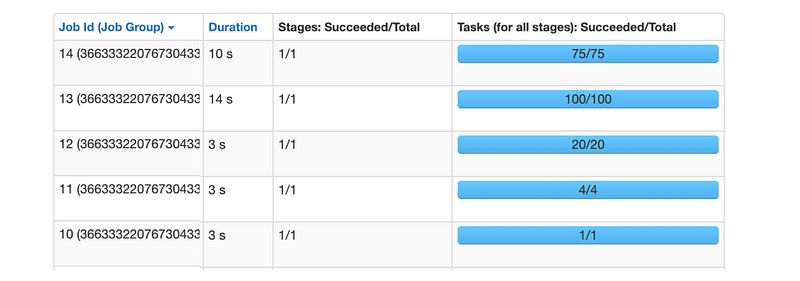
Also notice that number of tasks in each of these jobs is different. The first job (with job id = 10) had only one task! The next job run with four tasks, then 20, 100, and finally a job with 75 tasks was the last one. By the way, the cluster on which this was executed had 32 cores available, so 32 tasks could run in parallel.

The idea behind executing the query in multiple jobs is to avoid processing all input data. The show function returns only 20 rows by default (this can be changed by passing the n argument), so perhaps we can process only one partition of the data to return 20 rows. This is why Spark first runs a job with only one task that will process just one partition of the data hoping to find 20 rows that are required for the output. If Spark doesn’t find these 20 rows, it will launch another job that will process another four partitions (that’s why the second job has four tasks) and so the situation repeats, and Spark in each further job increases number of partitions that are processed until it finds the 20 required rows or all partitions are processed.

This is an interesting optimization that makes sense especially if your dataset is very large (contains many partitions) and your query is not very selective, so Spark can process really only the first few partitions to find the 20 rows. On the other hand, if your query is very selective and you are for example looking for a single row (which may not even exist) in a very big data set, it might be more useful to use the collect function which will use the full potential of the cluster from the beginning and process all data in one job because, in the end, all partitions will have to be processed anyway (if the record doesn’t exist).

7. How to make sure a User Defined Function is executed only once?

It is a known fact that user-defined functions (UDFs) are better to be avoided if they are not necessary because they bring some performance penalty (how big the penalty is, depends on whether the UDF is implemented in scala/java or python). What is not so obvious though, is that if the UDF is used, it might be executed more times than expected and so the overhead becomes even bigger. This can be however avoided and thus the overall penalty will be mitigated. Let’s see a simple example:

@udf('long')
def add_one(x):
    return x + 1

(
    spark.range(10)
    .withColumn('increased', add_one(col('id')))
    .filter(col('increased') > 5)
).explain()

In this example, we create a simple UDF that we use to add a new column to the DataFrame and next we filter based on this column. If we check the query plan by calling explain we will see:

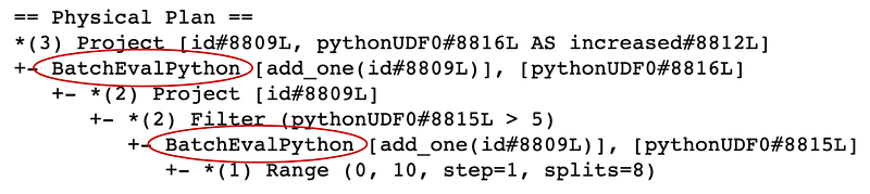
As you can see the BatchEvalPython operator is in the plan twice which means that Spark will execute the UDF twice. Obviously, this is not the most optimal execution plan, especially if the UDF becomes a bottleneck, which is often the case. Fortunately, there is a nice trick how to make Spark call the UDF only once and it is by making the function non-deterministic (see in documentation):

add_one = add_one.asNondeterministic()

(
    spark.range(10)
    .withColumn('increased', add_one(col('id')))
    .filter(col('increased') > 5)
).explain()

Now, checking the query plan reveals that the UDF is called only once:

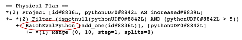
This is because Spark now thinks that the function is not deterministic, so calling it twice wouldn’t be safe since it could return a different result each time it is called. It is also good to understand that by doing this we are putting some constraints on the optimizer, which will now handle it in a similar way as other non-deterministic expressions, for example, filters will not be pushed through as we have seen with the collect_list function above.

8. UDF can destroy your data distribution

Not literally. But let me explain what I mean by this. Imagine a situation in which you want to join two tables which are bucketed and you also need to call a UDF on one of the columns. The bucketing will allow you to do the join without a shuffle, but you need to call the transformations in the correct order. Consider the following query:

(
  dfA.join(dfB, 'user_id')
  .withColumn('increased', add_one('comments'))
).explain()

Here we are joining two tables which are bucketed on the user_id column to the same number of buckets and we apply a UDF (add_one) on one of the columns from dfA. The plan looks as follows:

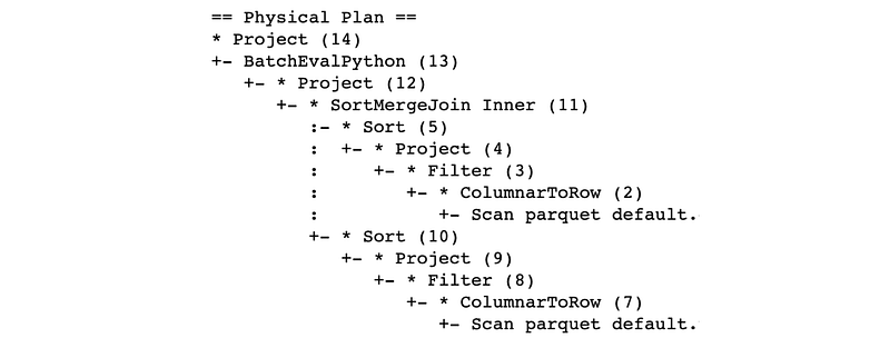
Here as you can see everything is fine because the plan has no Exchange operator and the execution will be shuffle-free, this is exactly what we need and it is because Spark is aware of the distribution of the data and can use it for the join.

On the other hand, let’s see what happens if we apply the UDF first and do the join after it:

(
  dfA
  .withColumn('increased', add_one('comments'))
  .join(dfB, 'user_id')
).explain()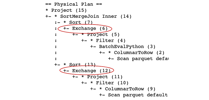

Now the situation changed and we have two Exchange operators in the plan, which means that Spark will now shuffle both DataFrames before the join. It is because calling the UDF removed the information about the data distribution and Spark now doesn’t know that the data is actually distributed well and it will have to shuffle it to make sure the partitioning is correct. So calling the UDF doesn’t really destroy the distribution but it removes the information about it, so Spark will have to assume that the data is distributed randomly.

Conclusion

In this article, we went over some examples of Spark features which may not be so obvious, or which are easy to forget when composing the queries. Improper use of some of them can lead to a bug in your code, for example, if you forget that sorting a window will change your frame, or that some functions will produce null if some of the input arguments are nulls (like the concat function). In some examples, we have also seen simple optimization tricks such as that making a UDF non-deterministic can avoid executing it twice, or calling the UDF after the join can save you from the shuffle if the tables are bucketed (or distributed according to some specific partitioning).

We have also seen that using SQL functions is sometimes more flexible than the DSL functions, one particular example of this is the array_sort which in SQL allows you to specify the comparator function to achieve custom sorting logic.