Dickey Fuller Direct Estimation — Speed up to 50x Test Statistic Computation

Avoid unnecessary regressions and matrix inversions by directly estimating the Dickey-Fuller test statistic through the correlation coefficient.

The Dickey-Fuller test is perhaps the most well-known among stationarity (unit root) tests in time series analysis. The computation procedure for the test relies on linear regression results for the concrete formulation of the statistic. However, linear regression requires matrix inversions, which can be computationally intensive and even numerically unstable.

In this story, we will explore the math behind OLS (ordinary least squares) and use such analysis to derive a closed-form expression for the Dickey-Fuller test statistic (using 1 time lag and a constant). The resulting expression only uses a correlation coefficient, there are no matrix inversions or computationally intensive operations. This can speed computations up to 50x.

Table of contents

• Closed-form expression derivation
• Closed-form expression result
• Sanity Check
• Speed Test
• p-values
• Final Words

Closed-form expression derivation

If you want to skip the mathematical details, scroll to the next section, no harm done.

For those of you still here, let us first enunciate the problem formally. The Dickey-Fuller test (non-augmented) autoregressive model specification up to one lag and a constant is:

with ε i.i.d, this equation can be cast into a form where the time series increment is explicit:

α, β and their variances are estimated through OLS.

The Dickey-Fuller test statistic is defined as:

We could perform OLS regression numerically, get β and its variance and call it a day. This would involve a matrix inversion and matrix multiplications which are computationally taxing. So we are not going to do that.

The other road we could take is doing the math. It seems that nowadays I spend most of my time crunching numbers on the computer and almost no time on the blackboard doing the actual math. In this case, doing the math does pay off.

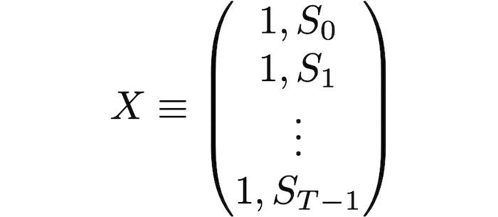
First, we will formulate our regression in terms of matrices and vectors as

where S_d is a vector of dimension T made up from the differences of S,

and X is a Tx2 matrix

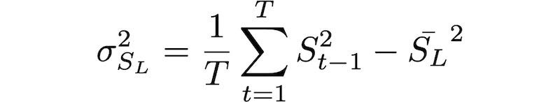
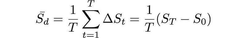
Let S_L be a T dimensional vector with the lagged time series S, then the following relationships hold:

• the mean of S_L:

• the variance of S_L:

• the mean of S_d:

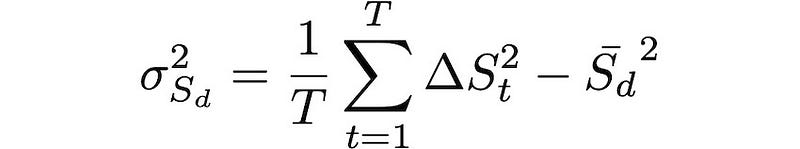
• the variance of S_d:

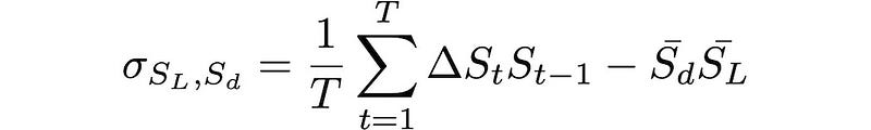
• the covariance of S_L and S_d:

Note that we do not use Bessel’s correction because the resulting equations would get a larger number of terms. When in doubt go for the result that yields the most beautiful mathematical expression. You could try it yourself, follow the next steps using Bessel’s correction for the variances.

The OLS estimator in matrix form is:

where T superscript denotes matrix transpose. We have then

its inverse:

and

Hence,

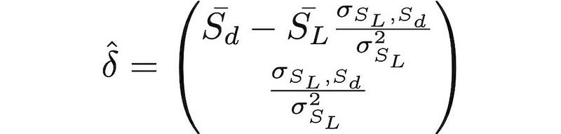
i.e.

where ρ is the Pearson correlation coefficient between the lagged series and the differenced series, and

Note that even if we had use Bessel’s correction for the variances, the results for α and β would remain unchanged.

Now we need to get the variance of β. From OLS we have that the covariance matrix of δ is:

Then the variance of β is:

where

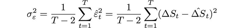
is the variance of the regression residuals. Note that we have used T-2 instead of T in the denominator because there are only only T-2 degrees of freedom for the residuals in OLS, since the two constraints hold:

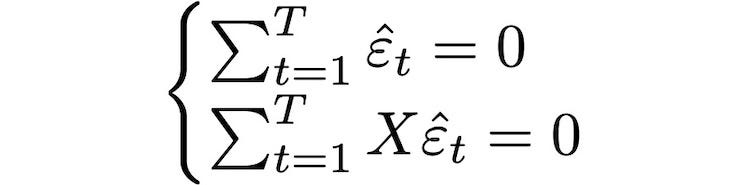
i.e. by construction the mean of the residuals is zero and the covariance between the regressors and the residuals is zero.

Then, expanding the equation for the variance of the residuals and noting that the estimation of the time series differences is:

we get that:

This result would have been a lot messier if we had used Bessel’s correction for the variances.

Then we can express the variance for β as

Finally, after all our hard work we can write the closed form for the Dickey-Fuller test statistic:

Closed-form expression result

The result for the closed-form expression of the Dickey-Fuller test statistic is:

where T+1 is the sample size of our data and ρ is the correlation coefficient between the lagged time series (sample size T) and the differenced time series (sample size T).

The only thing we need to compute is a correlation coefficient, which is more efficient than computing OLS. This becomes handy in optimization routines and in real-time analysis of time series, where each millisecond counts.

Sanity check

In this section, we will compare our results with the results obtained from the Statsmodels (Python) library. Let us define our functions for the Dickey-Fuller test statistic:

We will use an AR(1) unit root process with standard normal increments (Brownian motion) to conduct our tests:

Now, we get an estimate of the relative mean error of our direct Dickey-Fuller estimation and the OLS approach (Statsmodels), i.e. |DF_statmodels — DF_direct| / | DF_direct |. This is precisely what the next function accomplishes. It runs “n_tests” with random Brownian motions and returns an array with the differences.

Running the tests and plotting:

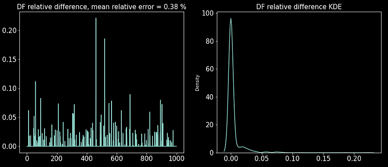
Note that your results will be different as this test is randomized. But for a time series of sample size 10,000 the relative mean error is around 1%. So our sanity check is indeed a success. There is, however, a slight difference between the two estimation approaches in some trials, this is due numerical instability caused by the unit root process in the estimation approaches. Nevertheless, it is something we can live with considering the increased computational efficiency.

Speed Tests

Now the best part. In this section, we will compare the speed between the OLS approach (Statsmodels) and the direct estimation of the Dickey-Fuller test. The following code performs the time test for any of the two functions (approaches).

Running the tests for a sample size range of 100 to 100,000 and plotting:

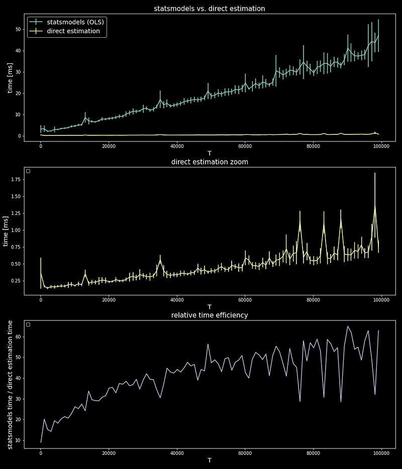
We can see that for large sample size time series the boost in speed is around 50x, but even for smaller sample sizes the is about 10x. So indeed, doing the math paid off.

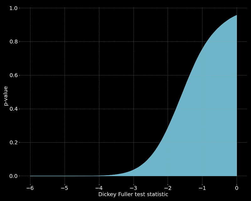
p-values

In this section, we will code a class to get p-values for the Dickey-Fuller test direct estimation. No statistical tool is complete without its p-values. We will do a Monte Carlo simulation using the AR(1) unit root process as described (and coded) above.

Note that in this class we use the “get_DF” function and the “get_unit_root_proc” from the previous sections.

As an example, we use the DFProbTable object to get P values for T=500 :

Final Words

The math in this story was a bit long, to say the least, but in the end, we got a result that was worth it. The formulation of the Dickey-Fuller statistic presented here is not only useful for optimizing computation efficiency but also to understand the statistic in another way.

There is also a lesson to be learned: sometimes as data scientists, it is very easy to use libraries and model everything without much understanding of the underlying mathematics. Nevertheless, it is a good idea to go deeper into the math, not just as a learning exercise but also as a way to get new and different insights. A little knowledge is a dangerous thing.

References

[1] M. L. de Prado, D. Leinweber, Advances in cointegration and subset correlation hedging methods (2012), Journal of Investment Strategies, Vol. 1, №2, pp. 67–115

[2]https://web.stanford.edu/~mrosenfe/soc_meth_proj3/matrix_OLS_NYU_notes.pdf

[3] http://web.vu.lt/mif/a.buteikis/wp-content/uploads/PE_Book/3-2-OLS.html

I hope this story was useful to you. If I missed anything, please let me know. Follow me on Medium if you would like more stories like this.

Liked the story? Become a Medium member through my referral link and get unlimited access to my stories and many others.