Summary

This guide illustrates the use of Fast Fourier Transform (FFT) in Python to denoise time series data by decomposing a noisy signal into its frequency components, identifying noise, and filtering it out to restore the original signal.

Abstract

The article presents a step-by-step approach to denoising time series data using Fast Fourier Transform (FFT) in Python. It begins by creating a synthetic dataset composed of three sinusoidal patterns with distinct frequencies, to which random noise is added. The noisy signal is then processed using FFT to identify the frequency components and isolate the noise. The Power Spectral Density (PSD) is calculated to determine the distribution of signal power across frequencies, allowing for the identification of dominant frequencies and noise. A threshold is set to filter out the noise components, and an Inverse FFT is applied to reconstruct the denoised signal. The process demonstrates the effectiveness of FFT in cleaning time series data, which is crucial for accurate analysis in various scientific and engineering fields.

Opinions

The author emphasizes the importance of FFT as an efficient algorithm for decomposing signals into their frequency components, which is essential for signal processing tasks.
The use of a synthetic dataset with known frequency components allows for a clear demonstration of the effectiveness of FFT in denoising.
By comparing the noisy and clean data, the article highlights the visual impact of noise on time series data and the improvement after applying FFT.
The article suggests that setting a threshold for filtering frequencies based on their power is a subjective decision that can significantly affect the outcome of the denoising process.
The author's choice to plot both the time domain and frequency domain representations of the data underscores the value of visual analysis in understanding signal processing results.
The conclusion reiterates the author's view that FFT is a powerful tool for data scientists, particularly for preprocessing time series data to enhance the accuracy of subsequent analysis.

Denoising data with Fast Fourier Transform — using Python

This guide demonstrates the application of Fast Fourier Transform (FFT) with Python. It involves creating a dataset comprising three sinusoidal patterns with varying frequencies, introducing random noise, and subsequently employing FFT to restore the series to its original form. This approach offers an intriguing method for cleaning time series data.

The Fast Fourier Transform (FFT) is an efficient algorithm for calculating the Discrete Fourier Transform (DFT) of a signal, allowing for the decomposition of a signal into its frequency components.

Step 1 — Create the dataset

First, we create a simple signal with three different frequencies (f1 = 75Hz, f2 = 120Hz, and f3 = 160Hz). Then, we create a combined signal, which is the sum of the three frequencies. Next, we create an array t with the sampling times at an interval dt. Finally, we create a copy of the combined signal and name it f_clean, which will be useful later for comparing the power of the FFT.

f1 = np.sin(2*np.pi*75*t) #Frecuency 75Hz
f2 = np.sin(2*np.pi*120*t) #Frecuency 120Hz
f3 = np.sin(2*np.pi*160*t) #Frecuency 160Hz
f = f1+f2+f3 # Combined signal
dt = 0.001
t = np.arange(0,1,dt)
f_clean = f

Step 2— Add random noise

Now we generate random noise with mean zero and standar deviation 1, scaled by an optional factor of 2.7, to finally add it to the combined series f .

noise = 2.7*np.random.normal(0,1,len(t))
f = f+noise

Now, we plot the combined series without noise and the combined series with noise, highlighting the disparity between the two. Moving forward, we will focus on the noisy series (or noisy data), to maintain a realistic representation.

# Customize size
plt.figure(figsize= (16,8))
# Noisy data
plt.plot(t, f, color='#0CBECD', linewidth=2, alpha=0.8, label='Noisy data')
# Clean data
plt.plot(t, f_clean, color='#010A0C', linewidth=3, label='Clean Data')

# labels and title
plt.xlabel('Time')
plt.ylabel('Amplitude')
plt.title('Denoising time series with FFT')
plt.legend(fontsize='medium')

# Set limits on the x-axis
plt.xlim(t[0], t[-1])

plt.show()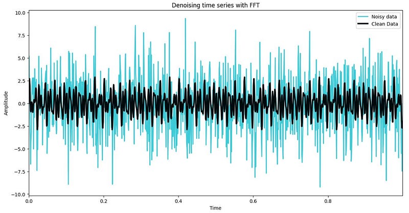

Step 3— Compute the Fast Fourier Transform

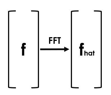
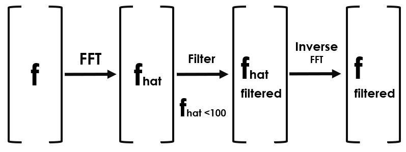
To calculate FFT, we use the numpy library with the fft.fft command, with the data to be transformed as the first parameter and the lenght as the second parameter, we store the result as fhat.

n = len(t)
fhat = np.fft.fft(f,n) # FFT transform

In summary, fhat represents the coefficients as a vector after the transformation. This provides us with the magnitude of the sine and cosine components, indicating which particular frequencies need attention. This helps us understand the frequency content of the signal and identify important frequency components.

The PSD (Power Spectral Density) is calculated from de Fourier coefficients (fhat) as the magnitud squared of coefficients (comples conjugate) divided by the length of the signal. This provides information about the distribution of the signal power in frequency domain, allowing the identification of dominant frequencies and understanding the relative contribution of each frequency.

Then we create a frequency vector representing all possible frequencies in the signal (freq). Next, we create a second vector , which contains the indices to acces frequencies within a desire range.

PSD = fhat * np.conj(fhat) / n # Power spectral density
freq = (1/(dt*n))*np.arange(n) # vector of all frequencies
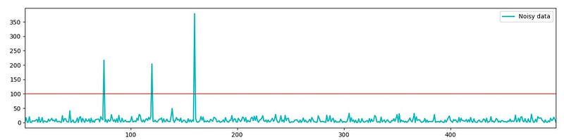
L = np.arange(1, np.floor(n/2), dtype = 'int') # indices

Now, we observe in the first graph the comparison between the noisy data and clean data. In the second graph, we see in the X-axis the frequency in Hertz and in the Y-Axis the Power Spectral Density.

fig, axis = plt.subplots(2,1, figsize=(16, 8))
plt.sca(axis[0])
plt.plot(t, f, color='#0CBECD', linewidth=1.5, label='Noisy data')
plt.plot(t,f_clean, color = '#010A0C', linewidth = 2, label = 'Clean Data')
plt.xlim(t[0], t[-1])
plt.legend()

plt.sca(axis[1])
plt.plot(freq[L], PSD[L], color = '#0CBECD', linewidth = 2, 
    label = 'Noisy data')
plt.xlim(freq[L[0]], freq[L[-1]])
plt.legend()

plt.show()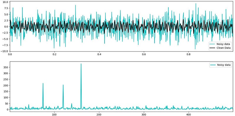

The power spectrum graph shows three prominent and clear peaks at 75, 120 and 160 Hertz, indicating that the noise in the noisy data is primarily concentrated at these frequencies. This allow us to filter out all the noise at these frequency peaks (setting a threshold of 100), where any Fourier coefficient with a magnitude greater than 100 will be filter. Then, we apply and Inverse Fourier Transform to revert to the original values without the noise at the identified peaks.

By setting a threshold of 100 on the power spectral graph, we identify 3 significant peaks to filter out and clean the data.

Step 4— Filtering data

Process for cleaning data with Fast Fourier Transform

indices = PSD > 100: It creates a boolean mask where each element of the Power Spectral Density (PSD) array that is greater than 100 is set to True, and the rest are set to False. PSDClean = PSD * indices: It multiplies each element of the Power Spectral Density array (PSD) by the corresponding element in the indices mask, effectively zeroing out all elements below the threshold of 100. fhat = indices * fhat: It applies the same masking to the Fourier coefficients (fhat), keeping only the coefficients corresponding to frequencies above the threshold. ffilt = np.fft.ifft(fhat): It performs an inverse Fast Fourier Transform on the modified Fourier coefficients to obtain the filtered time-domain signal.

indices = PSD > 100 # indices 
PSDClean = PSD*indices 
fhat = indices * fhat
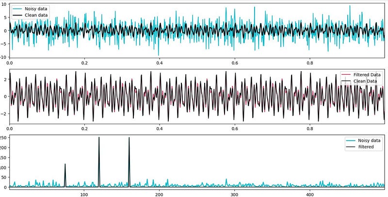
ffilt = np.fft.ifft(fhat)

Finally, we observe that the filtered data, reverted to its original values, closely match the real data we defined at the beginning, demonstrating that this method is a viable option for data cleaning.

fig, axis = plt.subplots(3,1, figsize = (16,8))
plt.sca(axis[0])
plt.plot(t,f, color = '#0CBECD', linewidth =1.5, label = 'Noisy data' )
plt.plot(t,f_clean, color = '#010A0C', linewidth= 2, label = 'Clean data' )
plt.xlim(t[0], t[-1])
plt.legend()


plt.sca(axis[1])
plt.plot(t, ffilt, color = '#c90a37', linewidth = 1.5, 
  label = 'Filtered Data', alpha = 0.8 )
plt.plot(t,f_clean, color = '#010A0C', linewidth=1.5, 
  label = 'Clean Data', alpha = 1)
plt.xlim(t[0], t[-1])
plt.legend() 


plt.sca(axis[2])
plt.plot(freq[L], PSD[L], color = '#0CBECD', 
  linewidth = 2, label = 'Noisy data')
plt.plot(freq[L], PSDClean[L], color = '#010A0C', 
  linewidth= 1.5, label= 'Filtered')
plt.xlim(freq[L[0]], freq[L[-1]])
plt.legend()
plt.show()

In conclusion, Fast Fourier Transform (FFT) for data cleaning is an effective technique, specially for time series data contaminated with noise. By identifying and filtering out noise components at specific frequency peaks, FFT enables us to restore the original signal, resulting in improved data quality and more accurate analysis. This approach offers a powerful tool for data scientist to preprocess and enhance times series data, ultimately leading to more robust and reliable insights.

Reference

Brunton, S. L., & Kutz, J. N. (Year). Data-Driven Science and Engineering: Machine Learning, Dynamical Systems, and Control