Deep Learning For Time Series Forecasting of Stock

The goal of this article is to develop and compare different approaches for time series.

Dependencies

import warnings
import numpy as np
import pandas as pd
import matplotlib.pyplot as plt
from keras import optimizers
from keras.utils import plot_model
from keras.models import Sequential, Model
from keras.layers.convolutional import Conv1D, MaxPooling1D
from keras.layers import Dense, LSTM, RepeatVector, TimeDistributed, Flatten
from sklearn.metrics import mean_squared_error
from sklearn.model_selection import train_test_split
import plotly.plotly as py
import plotly.graph_objs as go
from plotly.offline import init_notebook_mode, iplot

%matplotlib inline
warnings.filterwarnings("ignore")
init_notebook_mode(connected=True)

# Set seeds to make the experiment more reproducible.
from tensorflow import set_random_seed
from numpy.random import seed
set_random_seed(1)
seed(1)

First things first, we import necessary libraries and modules for building a convolutional neural network. It also sets up the environment for using plotly for visualisation and initalises seeds.

Loading Data

train = pd.read_csv('../input/demand-forecasting-kernels-only/train.csv', parse_dates=['date'])
test = pd.read_csv('../input/demand-forecasting-kernels-only/test.csv', parse_dates=['date'])

Here we read 2 csv files, one called train.csv and another one test.csv, and then convert the data column in each file into a date object. It then stores the contents of the files in the variable train and test.

Train Set

train.describe()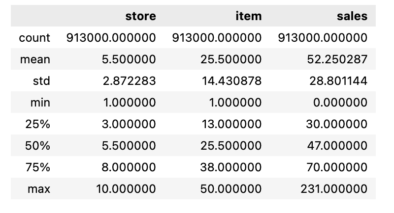

In this code we use the describe function on the train object and outputs a statistical summary of the data contained within the object.

train.head()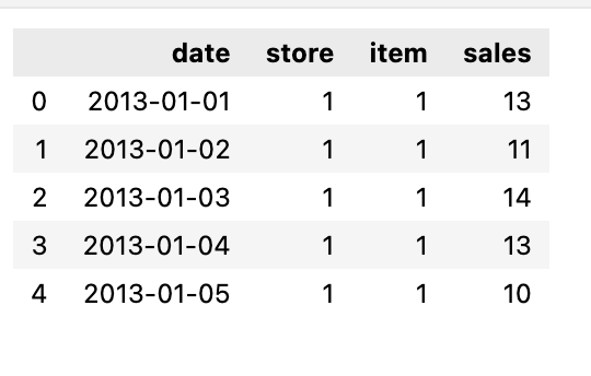

We need to print the first few rows of the train dataset.

Time Period of the Train Dataset

print('Min date from train set: %s' % train['date'].min().date())
print('Max date from train set: %s' % train['date'].max().date())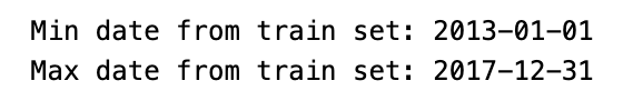

Using this code we print the minimum and maximum date from the date column of the train dataset. It uses the .min() and .max() functions to find the earliest and latest date, and then converts them to a date format before printing.

Before moving forward we need to find out what’s the time gap between the last day from training set from the last day of the test set, this will be out lag, the amount of day that we need to forecast.

lag_size = (test['date'].max().date() - train['date'].max().date()).days
print('Max date from train set: %s' % train['date'].max().date())
print('Max date from test set: %s' % test['date'].max().date())
print('Forecast lag size', lag_size)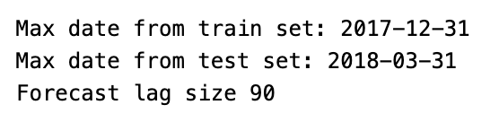

Using this code we can calculate the difference in days between the max date in the test and train datasets and points out the maximum dates from each dataset and the resulting forecast lag size.

Basic EDA

To explore the time series data first we need to aggregate the sales by day.

daily_sales = train.groupby('date', as_index=False)['sales'].sum()
store_daily_sales = train.groupby(['store', 'date'], as_index=False)['sales'].sum()
item_daily_sales = train.groupby(['item', 'date'], as_index=False)['sales'].sum()

This code takes a data set called train and groups it by date, store, and item, and then calculates the sum of sales for each date. It then returns the total daily sales, store-specific daily sales, and item-specific daily sales.

Overall Daily Sales

daily_sales_sc = go.Scatter(x=daily_sales['date'], y=daily_sales['sales'])
layout = go.Layout(title='Daily sales', xaxis=dict(title='Date'), yaxis=dict(title='Sales'))
fig = go.Figure(data=[daily_sales_sc], layout=layout)
iplot(fig)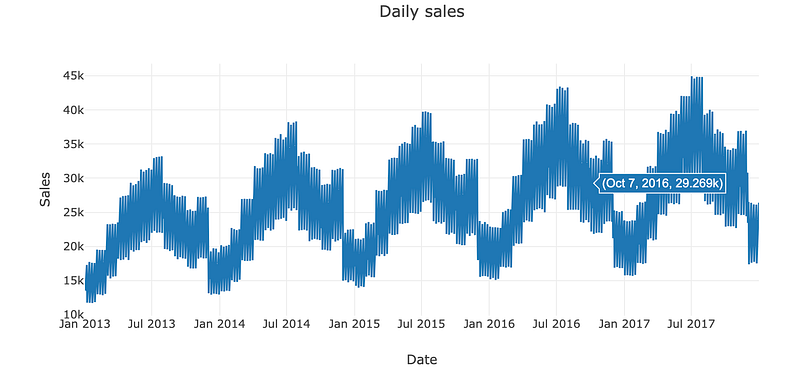

Using this particular code we can create a scatter plot of daily sales data, with the date on the x-axis and sales on the y-axis.

Daily Sales by Store

store_daily_sales_sc = []
for store in store_daily_sales['store'].unique():
    current_store_daily_sales = store_daily_sales[(store_daily_sales['store'] == store)]
    store_daily_sales_sc.append(go.Scatter(x=current_store_daily_sales['date'], y=current_store_daily_sales['sales'], name=('Store %s' % store)))

layout = go.Layout(title='Store daily sales', xaxis=dict(title='Date'), yaxis=dict(title='Sales'))
fig = go.Figure(data=store_daily_sales_sc, layout=layout)
iplot(fig)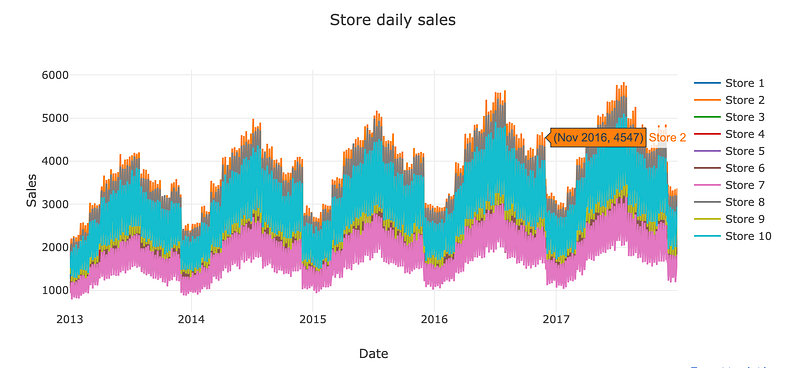

Here the code stores the daily sales data for different stores in a list and creates a scatter plot showing the sales over time for each store.

Daily Sales By Item

item_daily_sales_sc = []
for item in item_daily_sales['item'].unique():
    current_item_daily_sales = item_daily_sales[(item_daily_sales['item'] == item)]
    item_daily_sales_sc.append(go.Scatter(x=current_item_daily_sales['date'], y=current_item_daily_sales['sales'], name=('Item %s' % item)))

layout = go.Layout(title='Item daily sales', xaxis=dict(title='Date'), yaxis=dict(title='Sales'))
fig = go.Figure(data=item_daily_sales_sc, layout=layout)
iplot(fig)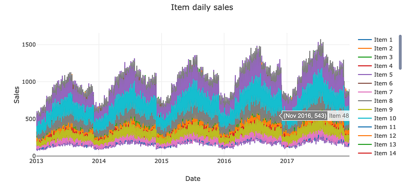

Sub Sample train set to get only the last year of data and reduce training time

train = train[(train['date'] >= '2017-01-01')]

Using this code we create a new variable called train and assign it to a subset of the original train data that contains only the rows where the date column is on or after January 1st 2017.

Rearrange dataset so we can apply shifts method

train_gp = train.sort_values('date').groupby(['item', 'store', 'date'], as_index=False)
train_gp = train_gp.agg({'sales':['mean']})
train_gp.columns = ['item', 'store', 'date', 'sales']
train_gp.head()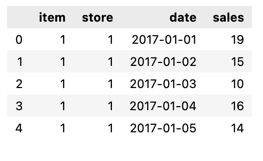

In this code we first sort the train dataset by the date column, then we group the data by the item, store, and date column. Then we calculate the mean of the sales column for each group and assign the result to the new dataframe called train_gp.

Transform the data into a time series problem

def series_to_supervised(data, window=1, lag=1, dropnan=True):
    cols, names = list(), list()
    # Input sequence (t-n, ... t-1)
    for i in range(window, 0, -1):
        cols.append(data.shift(i))
        names += [('%s(t-%d)' % (col, i)) for col in data.columns]
    # Current timestep (t=0)
    cols.append(data)
    names += [('%s(t)' % (col)) for col in data.columns]
    # Target timestep (t=lag)
    cols.append(data.shift(-lag))
    names += [('%s(t+%d)' % (col, lag)) for col in data.columns]
    # Put it all together
    agg = pd.concat(cols, axis=1)
    agg.columns = names
    # Drop rows with NaN values
    if dropnan:
        agg.dropna(inplace=True)
    return agg

This code takes a dataset, window size, and lag value. Then it create a supervised learning dataset from the input data by shifting the data to create a sequence of past and current timestamps, as well as a target timestamp for prediction. Then combines all the columns and drops any rows with missing values before returning the new dataset.

we are going to use the current timestep and the last 29 to forecast 90 days ahead

window = 29
lag = lag_size
series = series_to_supervised(train_gp.drop('date', axis=1), window=window, lag=lag)
series.head()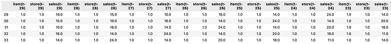

First we define 3 variables, window, with value 29, then lag with value of lag_size, then series, this is equal to result of a function call to series_to_supervised with parameters train_gp.drop(date,axis=1), window, and lag. After that it displays the tops few rows.

Remove Unwanted Column

columns_to_drop = [('%s(t+%d)' % (col, lag)) for col in ['item', 'store']]
for i in range(window, 0, -1):
    columns_to_drop += [('%s(t-%d)' % (col, i)) for col in ['item', 'store']]
series.drop(columns_to_drop, axis=1, inplace=True)
series.drop(['item(t)', 'store(t)'], axis=1, inplace=True)

Using this code we drop specific columns from a series of data based on a window and lag. It also drops additional columns related to the item and store being analysed.

Train/Validation Split

# Label
labels_col = 'sales(t+%d)' % lag_size
labels = series[labels_col]
series = series.drop(labels_col, axis=1)

X_train, X_valid, Y_train, Y_valid = train_test_split(series, labels.values, test_size=0.4, random_state=0)
print('Train set shape', X_train.shape)
print('Validation set shape', X_valid.shape)
X_train.head()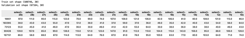

Using this code we create a label for a given column by adding a lag size, and then we create and drop a series for that label. Then we split the series into train and validation sets, with the train set being using sixty percent of the original series.

MLP for Time Series Forecasting

First we are going to use a multilayer perceptron model for NLP model, here our model will have input features equal to the window size. The only thing with MLP models it that the model don’t take the input as sequenced data, so for the model, it is just receiving inputs and don’t treat them as sequenced data, that may be problem since the model won’t see the data with the sequence patter that it has.

epochs = 40
batch = 256
lr = 0.0003
adam = optimizers.Adam(lr)

This code sets up the basics of our time series model.

model_mlp = Sequential()
model_mlp.add(Dense(100, activation='relu', input_dim=X_train.shape[1]))
model_mlp.add(Dense(1))
model_mlp.compile(loss='mse', optimizer=adam)
model_mlp.summary()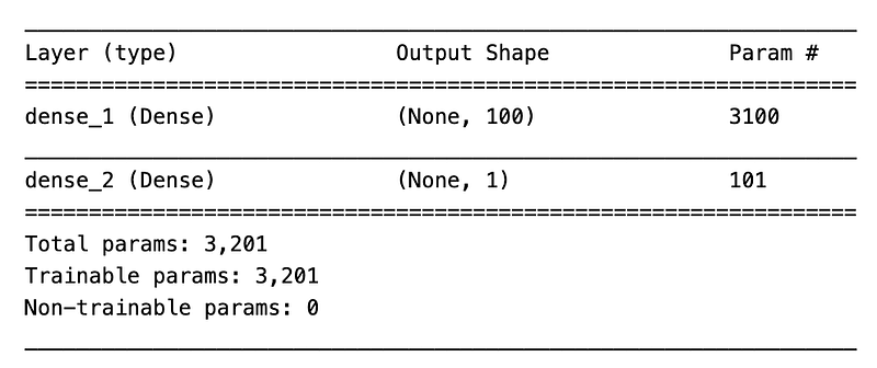

This code will create a neural network model using the sequential() function. It adds a layer with 100 neurons and a rectified linear unit, activation function, with an input dimension based on the shape of the training data. Then it adds another layer with one neuron. The model is then compiled using a mean squared error loss function and an adam optimizer.

mlp_history = model_mlp.fit(X_train.values, Y_train, validation_data=(X_valid.values, Y_valid), epochs=epochs, verbose=2)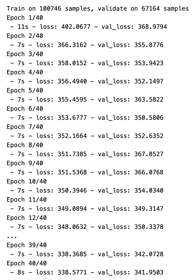

Through this code we train a multilayer perceptron NN model which is defined as model_mlp using the training data which is X_train and Y_train and then evalutes its performance using the validation data for a specified number of epochs, with a verbosity of level 2. The training history is then stored in the variable mlp_history.

LSTM For Time Series Forecasting

Now the lstm model actually sees the input data as a sequence, so it will be able to learn pattern from sequenced data better than the other ones, especially patterns from long sequence.

model_lstm = Sequential()
model_lstm.add(LSTM(50, activation='relu', input_shape=(X_train_series.shape[1], X_train_series.shape[2])))
model_lstm.add(Dense(1))
model_lstm.compile(loss='mse', optimizer=adam)
model_lstm.summary()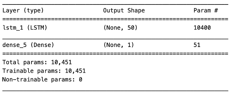

In this code we create a sequential model using LSTM layers with 50 units, a relu activation function, and an input shape based on the number of features in the training data. The it will add a dense layer with 1 unit and then compiles the model using the mean squared error loss function and the adam optimizer. It is also going to print the summary of our model.

lstm_history = model_lstm.fit(X_train_series, Y_train, validation_data=(X_valid_series, Y_valid), epochs=epochs, verbose=2)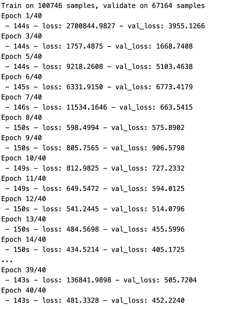

train the LSTM model using this code.

And this Is how you can use a basic LSTM for any prediction purposes.