Deep Learning: A Beginner’s Guide to Reccurent Neural Network (RNN) Architecture

Recurrent Neural Networks (RNNs) are powerful sequence models designed to capture patterns in sequential data. This article provides an introduction to RNN architecture, training processes, and the challenge of vanishing gradients.

INTRODUCTION

RNNs, also known as sequence models, are specifically designed to model patterns in sequential data. Unlike other deep learning models that don’t consider time as a factor, RNNs excel at capturing temporal dependencies and relationships across time.

While standard deep learning models process inputs at a single point in time and generate outputs based solely on those inputs, RNNs take into account the past information in the sequence. They have the capability to retain and utilize memory of past patterns to predict future occurrences.

For example, let’s say we have a sequence of stock prices over time. A regular deep learning model would only consider the current price to predict the future price. However, an RNN can incorporate the historical price data and fluctuations to make more accurate predictions.

Moreover, sequence models can predict multiple future values in a given sequence, if necessary. Additionally, there are bidirectional models that can even predict past values based on the information that comes after them in the sequence.

ARCHITECTURE

What does the architecture of an RNN look like?

Let’s explore a simplified recurrent neural network (RNN) structure. We’ll consider a time sequence consisting of four time steps: T1, T2, T3, and T4. These time steps can be non-equally spaced and can be conceptually separated, such as words in a sentence.

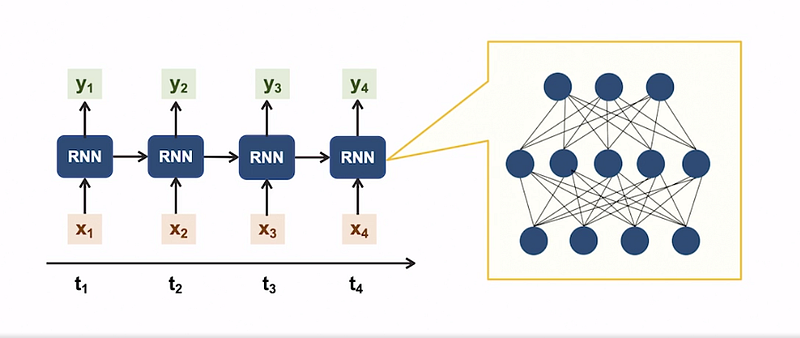
At each time step, there is a corresponding input: X1, X2, X3, and X4. These inputs are fed into the RNN. Although the RNN remains the same throughout all time steps, the input and output vary based on the specific time step. The RNN may generate an output at each time step, denoted as Y1, Y2, Y3, and Y4. This functioning is akin to a basic neural network. However, in addition to the output, the RNN also produces a hidden state that carries information from previous time steps to subsequent ones.

This hidden state, called memory, facilitates the propagation of information across time steps.

The RNN itself consists of multiple layers with nodes, weights, biases, inputs, and outputs. To summarize, the same neural network is utilized at each time step, featuring layers, nodes, weights, biases, and activation functions.

The network’s complexity can range from a simple single-layer network to a deep network with numerous layers. It possesses two inputs: the input from the current time step and the hidden state derived from the previous time step. Similarly, it has two outputs: the output for the current time step and the hidden state for the next time step.

TYPES OF RNN

There are various RNN architectures tailored for different use cases. Let’s examine these types and their applications.

1. Many-to-many RNN: Each time step has inputs and corresponding outputs. A prime example is speech recognition, where spoken words are translated into textual representations at each time step.
2. Many-to-one RNN: Inputs are present at each time step, but outputs are only generated after all inputs are provided in the final step. For instance, predicting the next day’s stock price based on historical prices or performing sentiment analysis on a sequence of text and producing a single sentiment output at the end.
3. One-to-many RNN: These architectures are less common, but an example is music synthesis. A single input is given, and the model generates a sequence of musical notes as the output.
4. Encoder-decoder RNN: Popular in transformers, this approach involves providing a set of inputs for the encoding phase, followed by generating a set of outputs from the decoder. The number of outputs may differ from the number of inputs. Machine translation, where an input sequence in one language is translated to another, exemplifies this architecture. It involves conveying the semantics rather than translating word-for-word. Text summarization is another example where the input is condensed into a shorter word count.
5. One-to-one RNN: This corresponds to a classical neural network with no hidden state available. The hidden states are what make RNNs unique and distinctive.

In summary, RNNs offer different architectural designs to accommodate diverse use cases, leveraging their hidden state capabilities to model sequential patterns effectively.

TRAINING OF RNN

Like with base training processes, training data for RNNs requires preparation and pre-processing before being used for model training. Weights and biases are initialized, and a forward propagation step is performed. Following forward propagation, prediction loss and cost are computed, serving as a basis for back-propagation and the subsequent update of weights and biases. Gradient descent is applied iteratively until the observed accuracy reaches the desired levels.

• What sets RNN training apart is its temporal nature. Training occurs in time steps, and each time step may generate an output depending on the architecture.
• Additionally, the computation of the hidden state and its propagation to future time steps play a crucial role in loss computation and back-propagation.
• When multiple outputs are involved, cumulative error is computed, and back-propagation is performed accordingly.

FORWARD PROPAGATION

Let’s explore the forward propagation process in RNNs in more detail. Similar to regular RNNs, we train an RNN model using multiple samples, each consisting of a sequence with multiple time steps. Although there are multiple time steps, the model remains the same throughout. It comprises layers, nodes, weights, biases, and activation functions, similar to regular neural networks. Additionally, a hidden state is computed and utilized for model training. The hidden state from the previous step contributes to both the current output and the next hidden state.

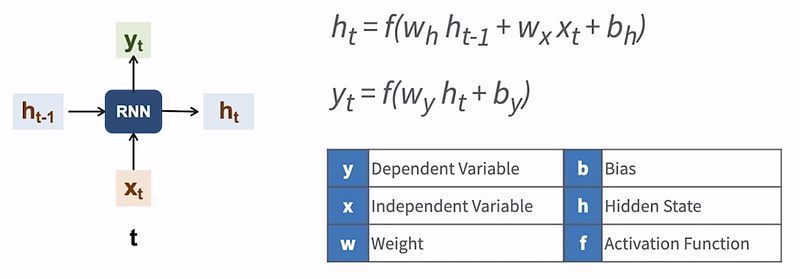
Let’s review the formulas used for these computations. At each time step, denoted as t, we have an input, x_t, which undergoes processing through a single RNN CELL. Furthermore, there is a hidden state, h_(t-1), obtained from the previous time step. We calculate h_t, the next hidden state, and y_t, the current output. For the initial time step, the previous hidden state is initialized as zeroes.

To compute h_t, we employ two sets of weights, W_h and W_x, and a bias, b_h. The formula for h_t is as follows:

h_t = activation_function(W_h * h_(t-1)+ W_x* x_t+ b_h)

For y_t, we use another set of weights, W_y, and a bias, b_y. The hidden state, h_t, is employed to compute y_t. Both the input, x_t, and the previous state, h_(t-1), influence the computation of y_t.

Unlike regular neural networks, which use a single set of weights and biases, RNNs employ three sets of weights and two sets of biases.

These values are randomly initialized and adjusted during the gradient descent process.

By leveraging these formulas and iterative training, RNNs can effectively capture sequential dependencies and learn from temporal data.

COMPUTING LOSS FUNCTION

The process of computing loss in RNNs is similar to that in regular neural networks.

We calculate the loss for each time step and then aggregate these losses across time steps to determine the overall loss for the given samples.

Subsequently, we compute the cost across a batch, consisting of multiple samples, and employ it for back propagation.

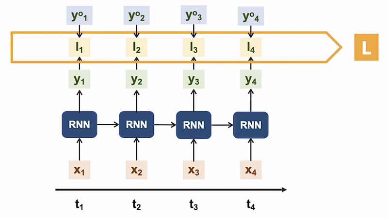
To illustrate, let’s consider an RNN with four time steps, each having four inputs and four corresponding outputs. During training, we possess actual target values for each output. We compute the difference between the predicted values and the actual values at each time step(l_t), resulting in individual loss values.

These losses are then combined across time steps to obtain the overall loss for the samples. Finally, the loss values across samples within a batch are utilized to calculate the cost.

By determining the loss and cost, we can assess the performance of the RNN model and utilize these metrics in subsequent steps such as back propagation and parameter updates.

BACKPROPAGATION

Now, we will utilize this cost function to calculate derivatives or deltas for both the hidden state and the output at each step. These derivatives represent the adjustments needed for various weights and biases in the network.

Subsequently, we compute the cumulative delta across all time steps, which we apply to update the weights and biases of the RNN model. This gradient descent process is repeated until the cost value reaches acceptable thresholds.

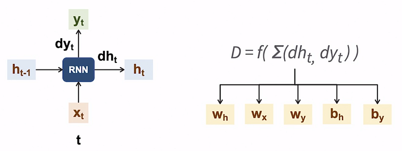
Let’s walk through this process step by step. Consider the network at time step t. First, we compute the derivative or delta, denoted as Dh_t for the hidden state h_t based on the computed cost. Similarly, we calculate the delta for the output, represented as Dy_t. For the sake of simplicity, we will not delve into the actual formula.

Next, we compute the cumulative delta by aggregating the deltas from individual time steps. This cumulative delta is then employed to adjust the weights and biases of the RNN model. Once the weights and biases have been adjusted, we continue with the gradient descent procedure to further train the model.

By iteratively performing back propagation and updating the model parameters, RNNs can learn from the training data, refine their predictions, and improve overall performance.

PREDICTIONS

Predictions with RNNs follow a straightforward approach similar to regular neural networks. The inputs provided to the RNN during prediction depend on the specific type of model being used. For instance, in time series predictions, the inputs may consist of a list of previous time steps, while in natural language processing, the inputs could be a sequence of text. The output of the RNN can be the next time step or another sequence of text, depending on the task at hand.

To make predictions, the input data undergoes the same preparation steps as the training data. Once prepared, the input data is fed into the RNN model, and predictions are generated.

THE PROBLEM OF VANISHING GRADIENT

In this section, we will address the issue of vanishing gradients in RNNs. To illustrate this, let’s consider an example of an RNN that takes the last four words in a sequence as input and predicts the next word. The inputs are denoted as x_1to x_4, while the output is represented as y.

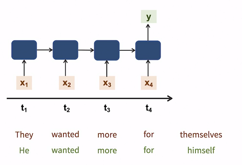
For instance, if we provide the input “they wanted more for,” we expect the model to predict the word “themselves.” However, a challenge arises in cases where similar input sequences exist. For example, if the input sequence is “he wanted more for,” the correct prediction should be “himself.”

In both sequences, the second, third, and fourth words are the same, but the output is dependent on the first word. In other words, the output Y at T4 is heavily influenced by the input at T1. This signifies a long-term dependency that must be accurately captured and propagated through the hidden states.

In a regular RNN, the output at each time step is primarily influenced by the input at that particular time step. As the hidden state traverses through the network, the importance of input weights diminishes over time.

For example, at T2, the generated hidden state relies more on X1 and X2, with X1 having a higher weight. As we progress to T3, X3 carries a higher weight than X2, while X2 holds a higher weight than X1.

The weight of X1 diminishes and loses significance as the sequence progresses. Although this is suitable for many sequence models, where the next value heavily depends on the most recent previous values, there are cases where long-term dependencies need to be maintained.

To address this issue, we can explore two alternative architectures that effectively tackle this problem and allow for the preservation of long-term dependencies in RNNs.

In conclusion, Recurrent Neural Networks (RNNs) offer a powerful architecture for modeling sequential data, capturing temporal dependencies, and retaining memory of past patterns. With various RNN types tailored to different use cases, training processes, and prediction methods, RNNs provide a versatile framework for tackling a wide range of tasks. Despite the challenge of vanishing gradients, alternative architectures exist to preserve long-term dependencies and enhance the effectiveness of RNNs in capturing complex sequential patterns.