Decision Tree from Scratch in Python

Decision trees are among the most powerful Machine Learning tools available today and are used in a wide variety of real-world applications from Ad click predictions at Facebook¹ to Ranking of Airbnb experiences. Yet they are intuitive, easy to interpret — and easy to implement. In this article we’ll train our own decision tree classifier in just 66 lines of Python code.

What is a decision tree?

Decision trees can be used for regression (continuous real-valued output, e.g. predicting the price of a house) or classification (categorical output, e.g. predicting email spam vs. no spam), but here we will focus on classification. A decision tree classifier is a binary tree where predictions are made by traversing the tree from root to leaf — at each node, we go left if a feature is less than a threshold, right otherwise. Finally, each leaf is associated with a class, which is the output of the predictor.

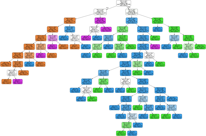
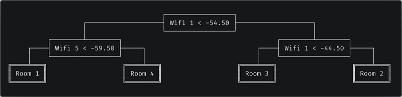
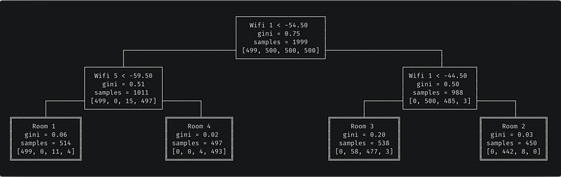
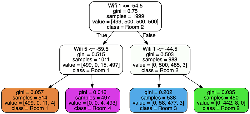
For example consider this Wireless Indoor Localization Dataset.² It gives 7 features representing the strength of 7 Wi-Fi signals perceived by a phone in an apartment, along with the indoor location of the phone which can be Room 1, 2, 3 or 4.

+-------+-------+-------+-------+-------+-------+-------+------+
| Wifi1 | Wifi2 | Wifi3 | Wifi4 | Wifi5 | Wifi6 | Wifi7 | Room |
+-------+-------+-------+-------+-------+-------+-------+------+
|  -64  |  -55  |  -63  |  -66  |  -76  |  -88  |  -83  |   1  |
|  -49  |  -52  |  -57  |  -54  |  -59  |  -85  |  -88  |   3  |
|  -36  |  -60  |  -53  |  -36  |  -63  |  -70  |  -77  |   2  |
|  -61  |  -56  |  -55  |  -63  |  -52  |  -84  |  -87  |   4  |
|  -36  |  -61  |  -57  |  -27  |  -71  |  -73  |  -70  |   2  |
                               ...

The goal is to predict which room the phone is located in based on the strength of Wi-Fi signals 1 to 7. A trained decision tree of depth 2 could look like this:

Gini impurity

Before we dive into the code, let’s define the metric used throughout the algorithm. Decision trees use the concept of Gini impurity to describe how homogeneous or “pure” a node is. A node is pure (G = 0) if all its samples belong to the same class, while a node with many samples from many different classes will have a Gini closer to 1.

More formally the Gini impurity of n training samples split across k classes is defined as

where p[k] is the fraction of samples belonging to class k.

For example if a node contains five samples, with two of class Room 1, two of class Room 2, one of class Room 3 and none of class Room 4, then

CART algorithm

The training algorithm is a recursive algorithm called CART, short for Classification And Regression Trees.³ Each node is split so that the Gini impurity of the children (more specifically the average of the Gini of the children weighted by their size) is minimized.

The recursion stops when the maximum depth, a hyperparameter, is reached, or when no split can lead to two children purer than their parent. Other hyperparameters can control this stopping criterion (crucial in practice to avoid overfitting), but we won’t cover them here.

For example, if X = [[1.5], [1.7], [2.3], [2.7], [2.7]] and y = [1, 1, 2, 2, 3] then an optimal split is feature_0 < 2, because as computed above the Gini of the parent is 0.64, and the Gini of the children after the split is

You can convince yourself that no other split yields a lower Gini.

Finding the optimal feature and threshold

The key to the CART algorithm is finding the optimal feature and threshold such that the Gini impurity is minimized. To do so, we try all possible splits and compute the resulting Gini impurities.

But how can we try all possible thresholds for a continuous values? There is a simple trick — sort the values for a given feature, and consider all midpoints between two adjacent values. Sorting is costly, but it is needed anyway as we will see shortly.

Now, how might we compute the Gini of all possible splits?

The first solution is to actually perform each split and compute the resulting Gini. Unfortunately this is slow, since we would need to look at all the samples to partition them into left and right. More precisely, it would be n splits with O(n) operations for each split, making the overall operation O(n²).

A faster approach is to 1. iterate through the sorted feature values as possible thresholds, 2. keep track of the number of samples per class on the left and on the right, and 3. increment/decrement them by 1 after each threshold. From them we can easily compute Gini in constant time.

Indeed if m is the size of the node and m[k] the number of samples of class k in the node, then

and since after seeing the i-th threshold there are i elements on the left and m–i on the right,

and

The resulting Gini is a simple weighted average:

Here is the entire _best_split method.

The condition on line 61 is the last subtlety. By looping through all feature values, we allow splits on samples that have the same value. In reality we can only split them if they have a distinct value for that feature, hence the additional check.

Recursion

The hard part is done! Now all we have to do is split each node recursively until the maximum depth is reached.

But first let’s define a Node class:

Fitting a decision tree to data X and targets y is done via the fit() method which calls a recursive method _grow_tree():

Predictions

We have seen how to fit a decision tree, now how can we use it to predict classes for unseen data? It could not be easier — go left if the feature value is below the threshold, go right otherwise.

Train the model

Our DecisionTreeClassifier is ready! Let’s train a model on the Wireless Indoor Localization Dataset:

As a sanity check, here’s the output of the Scikit-Learn implementation:

Complexity

It’s easy to see that prediction is in O(log m), where m is the depth of the tree.

But how about training? The Master Theorem will be helpful here. The time complexity of fitting a tree on a dataset with n samples can be expressed with the following recurrence relation:

where, assuming the best case where left and right children have the same size, a = 2 and b = 2; and f(n) is the complexity of splitting the node in two children, in other words the complexity of _best_split. The first for loop iterates on the features, and for each iteration there is a sort of complexity O(n log n) and another for loop in O(n). Therefore f(n) is O(k n log n) where k is the number of features.

With those assumptions, the Master Theorem tells us that the total time complexity is

This is not too far from but still worse than the complexity of the Scikit-Learn implementation, apparently in O(k n log n). If someone knows how this is possible, please let me know in the comments!

Complete code

The complete code can be found on this Github repo. And just for fun here is, as promised, a version stripped down to 66 lines.

¹ Xinran He, Junfeng Pan, Ou Jin, Tianbing Xu, Bo Liu, Tao Xu, Yanxin Shi, Antoine Atallah, Ralf Herbrich, Stuart Bowers, and Joaquin Quiñonero Candela. 2014. Practical Lessons from Predicting Clicks on Ads at Facebook. In Proceedings of the Eighth International Workshop on Data Mining for Online Advertising (ADKDD’14). ACM, New York, NY, USA, , Article 5 , 9 pages. DOI=http://dx.doi.org/10.1145/2648584.2648589

² Jayant G Rohra, Boominathan Perumal, Swathi Jamjala Narayanan, Priya Thakur, and Rajen B Bhatt, ‘User Localization in an Indoor Environment Using Fuzzy Hybrid of Particle Swarm Optimization & Gravitational Search Algorithm with Neural Networks’, in Proceedings of Sixth International Conference on Soft Computing for Problem Solving,2017, pp. 286–295.

³ Breiman, Leo; Friedman, J. H.; Olshen, R. A.; Stone, C. J. (1984). Classification and regression trees. Monterey, CA: Wadsworth & Brooks/Cole Advanced Books & Software.