Deciphering Signals: The Transformative Power of the Fast Fourier Transform in Digital Signal Processing

Introduction

The Fast Fourier Transform (FFT) is a fundamental algorithm in the field of digital signal processing and computational mathematics, with widespread applications ranging from audio signal analysis to image processing and beyond. This essay aims to unpack the FFT’s importance, its basic principles, and its applications, providing insights into why it has become an indispensable tool in various scientific and engineering domains.

In the world of complexity, the Transformative Power of the Fast Fourier Transform is our compass, revealing the hidden harmonies within the cacophony of data.

Origins and Evolution

The roots of the FFT trace back to the 18th century with Jean Baptiste Joseph Fourier’s introduction of the Fourier series, which laid the groundwork for representing functions as sums of sinusoids. However, it wasn’t until the mid-20th century that the FFT emerged as a practical computational algorithm, primarily attributed to the work of James W. Cooley and John W. Tukey in 1965. Their work revolutionized the way we compute the Discrete Fourier Transform (DFT), reducing the computational complexity from O(N2) to O(NlogN), where N is the number of data points. This leap in efficiency opened the doors to real-time processing of signals, which was previously unattainable with the computational resources of the time.

Principles of the Fast Fourier Transform

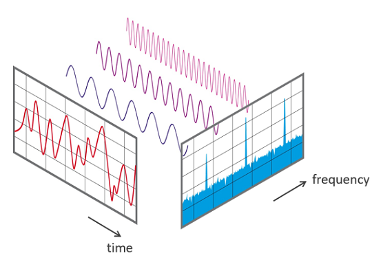
The FFT is an algorithm that efficiently computes the DFT of a sequence, or its inverse. The DFT is a mathematical transform used in converting spatial or temporal data into frequency domain data. The core idea behind the FFT is to decompose a DFT of any composite size N=N1​N2​ into many smaller DFTs, exploiting the periodicity and symmetry properties of the exponential factors in the DFT formula. This divide-and-conquer approach significantly reduces the number of arithmetic operations required, making the FFT incredibly efficient for large datasets.

Applications of the Fast Fourier Transform

The FFT’s applications are vast and varied. In telecommunications, it is used for modulating and demodulating signals, channel coding, and signal compression. In audio signal processing, the FFT allows for the analysis and enhancement of sound, noise reduction, and the development of music synthesis and recognition systems. In the field of image processing, the FFT is used for filtering, image analysis, and compression algorithms. Furthermore, the FFT is crucial in the numerical solution of partial differential equations, especially in simulations of physical phenomena such as fluid dynamics and electromagnetics.

Challenges and Future Directions

While the FFT is a powerful tool, it is not without its challenges. The accuracy of FFT-based methods can suffer from phenomena such as leakage, aliasing, and the picket fence effect. These issues necessitate careful windowing and sampling strategies. Moreover, the advent of quantum computing presents new challenges and opportunities for the FFT, potentially leading to even faster algorithms.

The FFT also continues to evolve, with research focused on optimizing its performance for modern computational architectures, including parallel processing and GPUs, and extending its applicability to non-uniformly sampled data through algorithms like the Non-uniform Fast Fourier Transform (NFFT).

Code

Implementing a Fast Fourier Transform (FFT) analysis in Python involves several steps, including generating a synthetic dataset, performing the FFT, and analyzing the results through metrics and plots. This approach provides a comprehensive understanding of how FFT operates and its application in signal processing. Below, I outline a complete example that includes:

1. Creating a Synthetic Dataset: Generating a signal composed of multiple sine waves.
2. Applying FFT: Computing the FFT of the dataset to convert it from the time domain to the frequency domain.
3. Metrics and Plots: Analyzing the transformed data through metrics and visualizations.
4. Interpretation: Offering insights into what the FFT reveals about the original dataset.

Step 1: Creating a Synthetic Dataset

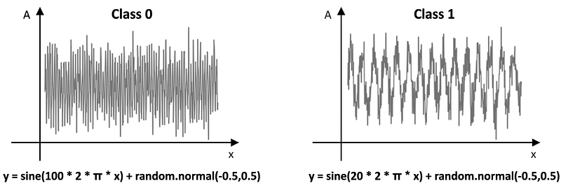
We’ll generate a synthetic signal that combines several sine waves with different frequencies and amplitudes to mimic a complex signal.

Step 2: Applying FFT

We use the numpy.fft.fft function to compute the FFT of our synthetic signal, allowing us to analyze its frequency components.

Step 3: Metrics and Plots

We’ll examine the amplitude spectrum of the signal to identify the frequency components. Plots will be generated to visualize both the original time-domain signal and its corresponding frequency-domain representation.

Step 4: Interpretation

The final step involves interpreting the results, focusing on how the FFT decomposes the signal into its constituent frequencies, revealing the signal’s complexity and underlying patterns.

Let’s implement this in Python:

import numpy as np
import matplotlib.pyplot as plt

# Step 1: Creating a Synthetic Dataset
# Parameters
fs = 500  # Sampling frequency
t = np.arange(0, 1, 1/fs)  # Time vector
f1, f2, f3 = 5, 50, 120  # Frequencies of the sine waves
A1, A2, A3 = 1, 0.5, 0.2  # Amplitudes of the sine waves

# Synthetic signal
signal = A1 * np.sin(2 * np.pi * f1 * t) + A2 * np.sin(2 * np.pi * f2 * t) + A3 * np.sin(2 * np.pi * f3 * t)

# Step 2: Applying FFT
fft_result = np.fft.fft(signal)
fft_freq = np.fft.fftfreq(signal.size, d=1/fs)

# Step 3: Metrics and Plots
# Plot the original signal
plt.figure(figsize=(14, 6))
plt.subplot(2, 1, 1)
plt.plot(t, signal)
plt.title('Original Signal')
plt.xlabel('Time (s)')
plt.ylabel('Amplitude')

# Plot the magnitude spectrum
plt.subplot(2, 1, 2)
plt.stem(fft_freq, np.abs(fft_result), 'b', markerfmt=" ", basefmt="-b")
plt.title('Magnitude Spectrum')
plt.xlabel('Frequency (Hz)')
plt.ylabel('Magnitude')
plt.xlim(0, fs/2)  # Nyquist limit
plt.tight_layout()
plt.show()

Interpretation

The first plot demonstrates the original signal in the time domain, showing how the signal varies over time, combining the effects of the three sine waves with different frequencies and amplitudes.

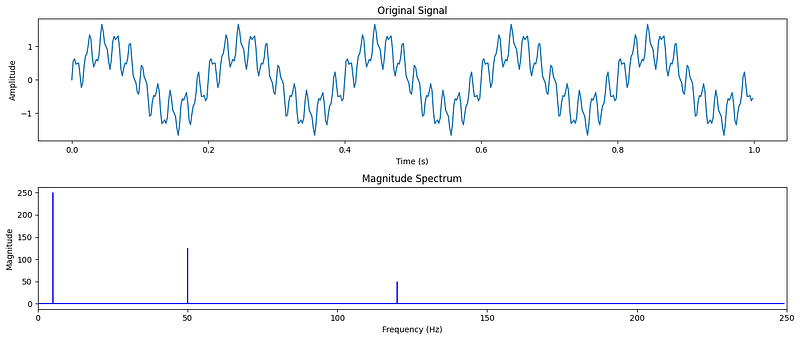
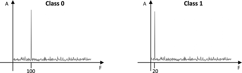
The second plot, the magnitude spectrum, reveals the frequency components present in the signal. Peaks in this plot correspond to the frequencies of the sine waves used to generate the signal. The magnitude of these peaks is proportional to the amplitudes of the respective sine waves in the time-domain signal.

Through this example, FFT’s power in signal processing is evident. It allows for the analysis of the frequency components of complex signals, providing insights that are not readily apparent in the time domain. This capability is invaluable across various applications, including audio signal processing, vibration analysis, and more sophisticated fields like telecommunications and astrophysics.

Conclusion

The Fast Fourier Transform stands as one of the most significant numerical algorithms ever developed, with a profound impact on our ability to process and understand the world through digital signals. Its efficiency and versatility have made it a cornerstone in many areas of science and engineering, facilitating advancements that were unimaginable before its development. As computational capabilities continue to grow, the FFT’s role in pushing the boundaries of what is possible in signal processing and beyond will undoubtedly persist and expand, continuing to fuel innovation across disciplines.