Dance with the arrays: A complete guide to NumPy

Welcome to the fascinating universe of NumPy, where Python’s numerical prowess takes center stage! In this blog, we’re about to unravel the secrets of NumPy — a toolkit that transforms mundane data handling into a captivating journey of efficiency and elegance.

Whether you’re a data scientist, coder, or just someone intrigued by the magic of numbers, NumPy is the key to unlocking a world where arrays become wizards, and numerical computing becomes an art. Join me as we embark on a short yet enthralling exploration into the heart of NumPy — your gateway to a more vibrant and efficient Python experience.

Before we start off by learning NumPy we should know what NumPy is and what are the advantages and use cases and why we are learning it in the first place.

What is NumPy?

NumPy, short for Numerical Python, is a powerful open-source library in Python that facilitates numerical operations on arrays and matrices. It provides an extensive set of functions for efficient data manipulation, mathematical computations, and scientific computing, making it a cornerstone in data science and analytics.

Advantages of NumPy

NumPy’s advantages lie in its ability to perform fast and efficient numerical computations in Python. With optimized array operations, it enhances code readability, facilitates complex mathematical manipulations, takes less space than lists and accelerates scientific computing, making it an indispensable tool for data analysis, machine learning, and scientific research.

Applications of Numpy

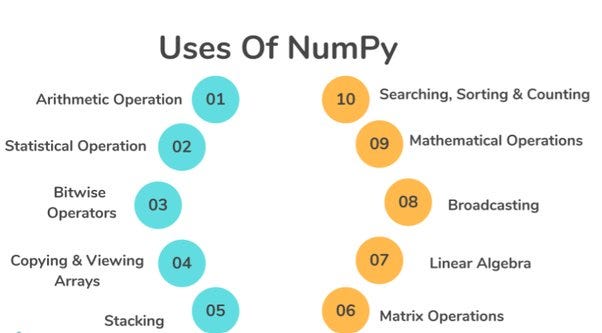
NumPy finds widespread applications in data science, machine learning, and scientific research. It empowers tasks like mathematical modeling, statistical analysis, image processing, and signal processing. NumPy’s versatile array operations make it a cornerstone in diverse fields requiring numerical computations in Python.

Now before we start using NumPy we need to install it first.

Installing NumPy

To install NumPy you need to open your command prompt and type in the following code

pip install numpy

Check NumPy version

You can also check the installed NumPy version by typing this:

print(np.__version__)

Importing NumPy

Before we use NumPy in our code we need to import it first. You can do that my using the following command

import numpy as np

Here np is short for NumPy and is the standard industry accepted short form that we generally use so that in all the commands we use from this library we can use np instead of typing numpy again and again.

Creating NumPy arrays

Now that we have successfully imported NumPy into our Jupyter Notebook we can start by creating arrays which are the the fundamental building blocks of NumPy.

# Creating a 1-D array
arr1 = np.array([1,2,3,4,5])
# Printing the array
print(arr1)
# Output: [1 2 3 4 5]

Here you can see that we have created a simple 1 dimensional array. Now one question that should be coming to your mind should be that how are arrays and different from lists? Allow me to answer that

Difference between lists and arrays

Lists in Python are versatile and can store different data types, while arrays, particularly NumPy arrays, are specialized and store homogeneous data, enabling efficient numerical computations and operations.

One thing to note is that array is also a type of datatype. You can check this by running the following command

type(arr1)
# Output: numpy.ndarray

Here we can see that the array that we made earlier is of the dataype array.

Now let’s try making a 2 dimensional array

# Creating a 2-D Array
arr2 = np.array([[1,2,3],[4,5,6]])
# Printing the array
print(arr2)
# Output:
'''[[1 2 3]
   [4 5 6]]'''

Checking the shape of the array

We can see how many rows and columns an array has using the shape function in NumPy

# Checking the shape of the arrays
print("Shape of arr1:", arr1.shape)
print("Shape of arr2:", arr2.shape)
# Output:
'''Shape of arr1: (5,)
   Shape of arr2: (2, 3)'''

Array Operations

NumPy allows you to perform various operations on arrays, such as element-wise addition, subtraction, multiplication, and more.

# Array addition 
result = arr1 + 10 # Element wise addition
print(result)
# Output: [11 12 13 14 15]

NumPy allows us to perform various mathematical functions as well.

# Performing sum operation on an array
sum_arr = np.sum(arr1)
print(sum_arr)
# Output: 15

# Performing mean operation on an array
mean_arr = np.mean(arr1)
print(mean_arr)
# Output: 3.0

# Performing squared function on an array
squared_arr = np.square(arr1)
print(squared_arr)
# Output:[ 1  4  9 16 25]

Array Attributes

Arrays have multiple attributes that gives us meaningful information about the arrays

# Array Attributes
print("Shape:", arr1.shape) # Gives shape of the array
print("Data Type:", arr1.dtype) # Gives datatypes of content in array
print("Number of Dimensions:", arr1.ndim) # Gives number of dimensions of array
print("Size:",arr1.size) # Gives number of elements in the array

''' Output:
Shape: (5,)
Data Type: int32
Number of Dimensions: 1
Size: 5'''

Some important NumPy functions

There are some useful functions that NumPy offers that you should be aware of. Allow me to guide you through them

np.zeros

Creates an array with the specified dimensions and fills the content with 0

zeros_arr = np.zeros((2, 3))
print(zeros_arr)
''' Output:
[[0. 0. 0.]
 [0. 0. 0.]]'''

np.ones

Similar to np.zeros but instead of 0 the data entered is 1

ones_arr = np.ones((3, 3))
print(ones_arr)
'''Output:
[[1. 1. 1.]
 [1. 1. 1.]
 [1. 1. 1.]]'''

np.arange

This function allows us to create an array where we can define the parameters such as how long the array should be and if we want to skip elements in it.

range_arr = np.arange(0, 10, 2)
print(range_arr)
# Output: [0 2 4 6 8]

np.linspace

Creates an array where it evenly creates an array of the defined length with equally spaced parameters depending on the number of parameters that we specify.

lin_space_arr = np.linspace(0, 1, 5)
print(lin_space_arr)
# Output: [0.   0.25 0.5  0.75 1.  ]

np.random.rand

Creates a random array with each value between 0 and 1

random_arr = np.random.rand(3, 3) 
print(random_arr)
''' Output:
[[0.6332693  0.86357605 0.95761624]
 [0.78824623 0.0314763  0.61329398]
 [0.82951793 0.79089062 0.2738745 ]]'''

copy

Allows us to copy the contents of one array into another array without changing the contents of the orignal array

arrr1 = arr1.copy()
print(arrr1)
# Output: [1 2 3 4 5]

np.identity

Allows us to create an identity matrix of a defined number of dimension

arr5 = np.identity(4)
print(arr5)
'''Output:
[[1. 0. 0. 0.]
 [0. 1. 0. 0.]
 [0. 0. 1. 0.]
 [0. 0. 0. 1.]]'''

Array Indexing

We can access various elements of the array using indexing

print("First element:", arr1[0])
print("Element at row 1, column 2:", zeros_arr[1, 2])
'''Output:
First element: 1
Element at row 1, column 2: 0.0'''

Array Slicing

We can slice arrays to extract subsets or parts of an array

subset_arr = arr1[1:3]
subset_matrix = zeros_arr[:, 1:]
print(subset_arr)
print(subset_matrix)
'''Output:
[2 3]

[[0. 0.]
 [0. 0.]]'''

Broadcasting

Broadcasting allows array operations on arrays of different shapes

arr10 = [1,2,3]
broadcast_result = arr10 + np.array([10, 20, 30])
print(broadcast_result)
# Output: [11 22 33]

Aggregation Functions

NumPy offers various aggregate functions as well. Let me introduce you to them

# Sum of array
arr11 = [1,2,3,4,5]
sum_arr = np.sum(arr11)
print(sum_arr)
# Output: 15

# Finding mean of each column
arr12 = np.ones((3,3))
mean_column = np.mean(arr12,axis = 0)
print(mean_column)
# Output: [1. 1. 1.]

# Finding the maximum element in an array
arr13 = [[1,2,3,4,5],
         [6,7,8,9,10]]
max_element = np.max(arr13)
print(max_element)
# Output: 10

Sorting in NumPy

NumPy also provide us with a convenient way to sort arrays

# Sorting an array
arr14 = [23,13,40,21,12]
sorted_array = np.sort(arr14)
print(sorted_array)
# Output: [12 13 21 23 40]

# Sorting an array in descending order
arr_descending = np.sort(arr14)[::-1]
print(arr_descending)
# Output: [40 23 21 13 12]

Searching in NumPy

NumPy allows us to search for elements in an array

arr15 = np.linspace(0,10,5)
index_of_value = np.searchsorted(arr15, 7.5)
print(index_of_value)
# Output: 3

Matrix Operations

NumPy allows us to perform various matrix operations on the array

# Dot product in a matrix
arr16 = np.ones((3,3))
arr17 = np.zeros((3,3))
matrix_product = np.dot(arr16, arr17)
print(matrix_product)
'''Output:
[[0. 0. 0.]
 [0. 0. 0.]
 [0. 0. 0.]]'''

# Transpose of a matrix
arr18 = [[1,2,3],
        [4,5,6]]
transpose_matrix = np.transpose(arr18)
print(transpose_matrix)
'''Output:
[[1 4]
 [2 5]
 [3 6]]'''

Singular Value Decomposition(SVD)

NumPy allows us to perform SVD. SVD is a factorization method that represents a matrix as the product of three matrices: A=UΣVT, where A is the original matrix, U is the left singular vectors matrix, ΣΣ is the diagonal matrix of singular values, and VT is the transpose of the right singular vectors matrix.

# Creating an example 2D array
arr19 = np.ones((3, 3))

# Performing SVD
u, s, vt = np.linalg.svd(arr19)

# Displaying the results
print("Original Matrix:")
print(ones_arr)

print("\nLeft Singular Vectors (U):")
print(u)

print("\nSingular Values (Sigma):")
print(np.diag(s))  # Diagonal matrix of singular values

print("\nRight Singular Vectors Transpose (V^T):")
print(vt)

'''Output:
Original Matrix:
[[1. 1. 1.]
 [1. 1. 1.]
 [1. 1. 1.]]

Left Singular Vectors (U):
[[-5.77350269e-01  8.16496581e-01 -1.75121059e-16]
 [-5.77350269e-01 -4.08248290e-01 -7.07106781e-01]
 [-5.77350269e-01 -4.08248290e-01  7.07106781e-01]]

Singular Values (Sigma):
[[3.00000000e+00 0.00000000e+00 0.00000000e+00]
 [0.00000000e+00 2.55806258e-17 0.00000000e+00]
 [0.00000000e+00 0.00000000e+00 2.11125548e-48]]

Right Singular Vectors Transpose (V^T):
[[-0.57735027 -0.57735027 -0.57735027]
 [ 0.81649658 -0.40824829 -0.40824829]
 [ 0.         -0.70710678  0.70710678]]'''

Generating random arrays

We can create random arrays with random data in them using NumPy

normal_dist = np.random.randint(0, 100, size=(3, 3))
print(normal_dist)
'''Output:
[[89  0  4]
 [25 25 97]
 [ 3 55 11]]'''

Note that the above generated array is random and may differ if you run this code yourself.

File Input/Output

NumPy allows us to write and store data into a txt file

np.savetxt('data.txt', ones_arr)
loaded_arr = np.loadtxt('data.txt')
# Output: A txt file is stored in the computer with a 3 x 3 ones matrix data

As we draw the curtains on our exploration of NumPy, take a moment to appreciate the invaluable insights you’ve gained in the realm of numerical computing. From the basics of array manipulation to the intricacies of singular value decomposition, you’ve navigated this journey with commendable proficiency. May the knowledge acquired serve as a cornerstone for your future endeavors in data science and scientific computing. As you move forward, let the principles of NumPy continue to be your reliable companion, ensuring accuracy and efficiency in your analytical pursuits.

Thank you for reading through this blog and I hope that you learnt something new by reading it.