Essential Math for Machine Learning: Gini Index and Entropy

Impurity Measures

This article is part of the series Essential Math for Machine Learning.

Introduction

Machine learning (ML) algorithms work by finding patterns in vast amounts of data. A core part of this process is making effective decisions about how to split datasets into meaningful categories or predictions. Impurity measures, specifically the Gini Index and Entropy, are indispensable tools for aiding these crucial decisions within ML models.

What are Impurity Measures?

Impurity measures gauge the degree of ‘mixed-up-ness’ or heterogeneity within a set of data. A pure dataset would contain elements belonging entirely to one class, and an impure dataset would have elements mixed from various classes. Decision trees, a fundamental machine learning algorithm, heavily rely on impurity measures to determine the best way to split a dataset at different points (nodes) of the tree.

Gini Index

The Gini Index measures the probability of incorrectly classifying a randomly selected element from a dataset if that element was labeled randomly according to the class distribution within the set. Imagine there is a box of balls of different colors, you know the number of each color, then you randomly pick a ball from the box without looking, then you guess its color based on the probability distribution, the Gini Index measures the probability of your guess is wrong.

Formula

Gini Index = 1 — Σ ( pi )²

Where:

• pi represents the probability of an element belonging to a particular class.

Explanation:

• Gini Index values range between 0 and 1.
• A Gini Index of 0 indicates a perfectly pure dataset (all elements belong to the same class).
• A Gini Index of 1 indicates the highest level of impurity (elements are evenly distributed across various classes).

Here’s a breakdown of why the Gini Index measures the probability of incorrectly classifying a randomly selected element from a dataset if that element was labeled randomly according to the class distribution within the set:

1. Random Selection: Imagine we select an element from the dataset without looking at its actual class label. This represents a “random” selection.

2. Random Labeling according to Class Distribution: Instead of assigning the correct class, we randomly decide its label based on how the classes are distributed in the dataset. For example, if our dataset has 60% “Class A” and 40% “Class B” elements, there’s a 60% chance we’ll randomly label our selected element as “Class A” and a 40% chance as “Class B”.

3. The Gini Index Calculation: Here’s where the Gini Index comes in. Recall the formula: Gini Index = 1 — Σ (pi)² (where pi is the probability of each class).

4. Probability of Misclassification: Focus on the ‘squaring’ part of the Gini Index calculation. If we randomly label our selected element, the squared probability of the assigned class actually represents the probability that we’ve assigned the correct class just by chance. Why? Suppose our label assignment aligns with the true distribution (say, 60% “A” and 40% “B”). then: There’s a 0.6 * 0.6 = 0.36 (36%) chance we randomly guessed “A” and were actually correct. There’s a 0.4 * 0.4 = 0.16 (16%) chance we randomly guessed “B” and were actually correct. Now, when we subtract the sum of these squared probabilities from 1, what we’re left with is the probability that our random guess was incorrect.

The Gini Index cleverly tells us how likely we are to misclassify an element if we just go around assigning labels randomly based on the dataset’s overall class proportions. So essentially, the Gini Index is a probability.

Minimum Gini Impurity Condition

Consider a scenario where all elements in a dataset belong to a single class, let’s say class k. This implies:

• pk = 1 (The probability of belonging to class k is 100%)
• pi = 0 (for all other classes i, where i ≠ k)

Substitute these probabilities into the Gini Index formula:

Gini Index = 1 — [(1)² + (0)² + … + (0)²] = 1–1 = 0

Maximum Gini Impurity Condition

Consider a scenario with ’n’ classes where each class has equal probability:

pi = 1/n (for all classes i)

Substitute pi = 1/n into the Gini Index formula:

Gini Index = 1 — Σ [(1/n)²] = 1 — (n * 1/n²) = 1–1/n

Consider the situation as the number of classes ’n’ increases towards infinity:

lim (n → ∞) [1–1/n] = 1

Entropy

Entropy, rooted in information theory, quantifies the level of uncertainty or randomness in a dataset. Entropy measures the length of optional encoding.

Formula

Entropy = — Σ pi * log2(pi)

Where:

• pi represents the probability of an element belonging to a particular class.

Explanation:

• Entropy values are non-negative.
• Entropy of 0 indicates perfect purity.
• Higher entropy values signify greater impurity.

Here’s how we can prove that the maximum entropy of a discrete probability distribution occurs when all outcomes are equally likely, and calculate the corresponding maximum value:

Assumptions

• Discrete Distribution: We are dealing with a finite set of ’n’ possible outcomes.
• Probabilities: pi represents the probability of the ith outcome (0 <= pi <= 1 for all i).
• Normalization: The probabilities of all outcomes must sum to 1 (Σ pi = 1).

Minimum Entropy Condition

Let’s consider the scenario where all elements in a dataset belong to one specific class, class k:

• pk = 1 (The probability of belonging to class k is 100%)
• pi = 0 (for all other classes i, where i ≠ k)

Substitute these probabilities into the Entropy formula:

H = — [(1 * log2(1)) + (0 * log2(0)) + … + (0 * log2(0))] = 0

The term log2(0) is undefined. However, in the context of information theory, the following convention applies: x * log2(x) approaches 0 as x approaches 0.

Maximum Entropy Condition

We will use the method of Lagrange multipliers along with the concept of concavity from calculus to demonstrate this maximality property.

1. Entropy Formula

Entropy (H) = — Σ [pi * log2(pi)]

2. Constraint

The probabilities must sum to 1: Σ pi = 1

3. Lagrange Multiplier

Introduce a Lagrange multiplier (λ) and form the Lagrangian function (L):

L = — Σ [pi * log2(pi)] + λ (Σ pi — 1)

4. Partial Derivatives

Calculate partial derivatives of L with respect to each pi and λ:

∂L / ∂pi = -[log2(pi) + 1] + λ ∂L / ∂λ = Σ pi — 1

5. Setting Derivatives to Zero

To find the maximum, we set the partial derivatives equal to zero:

• [log2(pi) + 1] + λ = 0 Σ pi — 1 = 0

6. Solving for pi

From the first equation: log2(pi) = -λ — 1. This implies pi = 2^(-λ — 1) for all i.

Since Σ pi = 1, we have: n * 2^(-λ — 1) = 1 Therefore, pi = 1/n for all i (all outcomes are equally likely).

7. Demonstrating Maximum

The Entropy function is concave. Combining this with the fact that we found a stationary point under the constraint (all pi equal), guarantees that this point is a global maximum.

8. Maximum Entropy Value

Substituting pi = 1/n back into the entropy formula:

H_max = — Σ [(1/n) * log2(1/n)] = — (n * (1/n) * -log2(n)) = log2(n)

The maximum entropy for a discrete distribution with ’n’ outcomes is log2(n), and it is achieved when all outcomes have equal probability (1/n).

Gini Index vs. Entropy in Machine Learning

Both the Gini Index and Entropy serve similar purposes in decision trees — guiding splits to create more homogeneous branches. They differ mainly in the way they calculate impurity:

• Meaning: Gini Index is a probability in the range of [0, 1], while entropy is a length in the range of [0, log2(n)] where n is the number of different classes.
• Computational Efficiency: Gini Index calculations tend to be slightly faster than Entropy.
• Interpretation: While they generally yield similar results, some practitioners find Gini Index slightly easier to interpret intuitively.

Implementing Gini and Entropy from Scratch

The code is available in this colab notebook.

import numpy as np
import matplotlib.pyplot as plt

def gini_index(p):
    return 1 - np.sum(p ** 2)

def entropy(p):
    p_log2_p = np.where(p > 0, p * np.log2(p), 0)
    return -np.sum(p_log2_p)

# Generate sample data with varying impurity
probabilities = np.linspace(0.01, 0.99, 50)  # Array from 0.01 to 0.99 for one class
data = np.array([probabilities, 1 - probabilities])  # Two classes

# Calculate Gini Index and Entropy
gini_values = [gini_index(p) for p in data.T]
entropy_values = [entropy(p) for p in data.T]

# Plotting
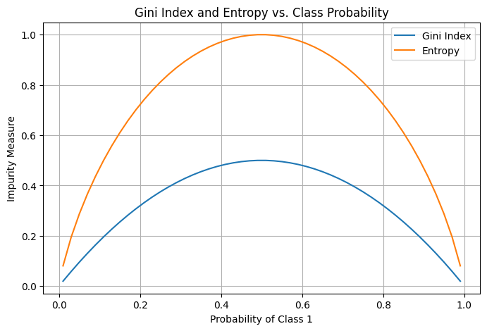
plt.figure(figsize=(8, 5))

plt.plot(probabilities, gini_values, label="Gini Index")
plt.plot(probabilities, entropy_values, label="Entropy")

plt.xlabel("Probability of Class 1")
plt.ylabel("Impurity Measure")
plt.title("Gini Index and Entropy vs. Class Probability")

plt.legend()
plt.grid(True)
plt.show()

Conclusion

In conclusion, the Gini Index and Entropy play a vital role in decision-making processes within machine learning models. By providing a numerical way to assess the purity of datasets, they guide algorithms towards creating effective classifications and predictions. Understanding how these measures work will enhance your ability to build smarter and more accurate machine learning solutions.