Critical Facts That Every Data Scientist Should Know — Part 1

Many data scientists are fantastic programmers but ignoring certain statistical facts can have very serious consequences.

Introduction

In this article, I want to explain to you some simple but at the same time critical concepts to avoid ending up like the machine above. In my experience, even seasoned data scientists sometimes don’t know or fully understand at least some of the topics I’m going to tell you about.

While not knowing the latest algorithm in vogue is generally harmless, having a partial understanding of some of the concepts described in this article is at the root of the most costly failures in data science.

having a partial understanding of some of the concepts described in this article is at the root of the most costly failures in data science

Each of the topics I will describe below could easily be and sometimes is, covered in a dedicated article. My goal here is to give you maximum return for minimum effort and to explain these often obscure concepts as simply as possible.

Due to the number of arguments covered, I have decided to divide this article into two parts, the second more advanced than the first:

Part 1

1. Introduction to the Use Case and the Confusion Matrix
2. Do You Really Want to Maximize Accuracy?
3. Precision, Recall and F1-Score
4. What Happens to Precision When the Class of Interest Becomes Less Frequent
5. Metrics for Imbalanced Classification

Part 2

1. Data Leakage, When Your Results Are Too Good to Be True
2. Interpretability and Simpson’s Paradox
3. How Sampling Bias Affects Your Model
4. Non-Stationarity and Covariate Shift
5. Observer Effect and Concept Drift

The graphs and results shown in this article can be reproduced and better understood using the associated Jupyter notebook easily run from Google Colab, I highly recommend you to try it!

Introduction to the Use Case and the Confusion Matrix

The first part of this article will focus on one of the most frequent problems in the world of data science: binary classification. From the Wikipedia page on Binary classification:

Binary classification is the task of classifying the elements of a set into two groups on the basis of a classification rule

Although in our examples we will have only two classes, practically all the arguments given apply equally in the case of multiclass classification.

To help the imagination, in this first part of the article I will use an example of a company that wants to use machine learning to understand if some of its customers are committing fraud, the problem that usually goes by the name of fraud detection.

We then define class 1/”positive” as the fraudsters and class 0/”negative” as the normal customers.

Since many of the metrics we’ll be using are easily calculated from the confusion matrix, before I start with the actual article, I’ll do a brief review of how it’s defined. If you’ve encountered this concept before feel free to skip this part. Let’s start by looking at the structure of this matrix:

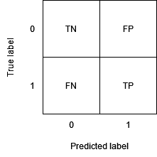
As we can see, the confusion matrix reports the four possible combinations between what is the actual class and what is the predicted class:

• True negative (TN): A negative that we predicted as such. In our case: a customer who committed no fraud and whom our model (correctly) did not report.
• False positive (FP): A negative that we predicted as a positive. In our case: a customer who committed no fraud and whom our model (mistakenly) reported.
• False negative (FN): A positive that we predicted as a negative. In our case: a customer who committed fraud and whom our model (mistakenly) did not report.
• True positive (TP): A positive that we predicted as such. In our case: a customer who committed fraud and whom our model (correctly) reported.

This is all we need before proceeding with the article, if you still had any doubt I suggest you look at the excellent Wikipedia page on confusion matrix.

Note: Sometimes the order of rows and columns is the reverse of the above, since this article is accompanied by a notebook to experiment with, I used the same convention used by the famous scikit-learn library (see the accompanying code).

Do You Really Want to Maximize Accuracy?

One of the most popular but also most misleading metrics used to measure performance in classification problems is accuracy.

• Accuracy (ACC): Percentage of times in which our model has predicted the correct class. Mathematically: ACC = (TP + TN) / (TP + TN + FP + FN).

Let’s imagine that we train two models to classify our customers into fraudsters and non-fraudsters, which model seems to perform better looking at the accuracy values below?

DummyClassifier accuracy: 90.91%
LogisticRegression accuracy: 77.82%

The name of the first model might make you suspect something, but just looking at the numbers it seems clear that DummyClassifier is performing better than LogisticRegression.

Is this really the case? Let’s look at the confusion matrices:

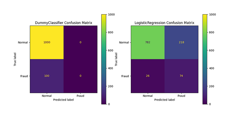
Actually, the DummyClassifier gives the correct prediction more times than the LogisticRegression (otherwise its accuracy would not be higher) but it NEVER predicts the fraud class. On the other hand, the LogisticRegression makes more mistakes but at least it helps us to identify 74 of the 100 frauds that our customers are committing.

What is this phenomenon due to? Let’s think first about the types of errors that are possible:

• My client is a fraudster and my model doesn’t realize it (false negative).
• My client is not a fraudster but my model thinks he is (false positive).

Accuracy gives equal weight to the two types of errors and, most importantly, does not care if our model is making “too many” errors of either type.

Accuracy […] does not care if our model is making “too many” errors of either type

Clearly, a model for identifying fraud that never reports a fraud is completely useless, as would be one that reports all customers as fraudsters, so we’d like metrics to help us know when the model is exaggerating one way or the other.

A question that could arise is: so in what cases do I have to think well before using accuracy as the main metric?

Accuracy tends to be high regardless of the goodness of the model when the classes are very unbalanced because, in this case, is enough to predict the most frequent class to get a very high accuracy.

Accuracy tends to be high regardless of the goodness of the model when the classes are very unbalanced because, in this case, is enough to predict the most frequent class to get a very high accuracy

In fact, our DummyClassifier is simply using the “most_frequent” strategy and so its predictions are always just “not fraud”, the most frequent class in the training dataset.

Precision, Recall and F1-Score

Let’s look at some classification metrics that solve one of the accuracy problems.

• Precision (or positive predictive value, PPV): Percentage of times in which the model is right when it has predicted class 1. E.g., if the model says “fraud” 100 times and the precision is 75%, on average it will be right in 75 cases, the other 25 are false alarms. Mathematically: PPV = TP / (TP + FP).
• Recall (or true positive rate, TPR): Percentage of the observations of class 1 that the model classifies as such. E.g. if between my customers there are 100 fraudsters and the recall is 75%, I will identify, on average, 75 of them, missing the other 25. Mathematically: TPR = TP / P = TP / (TP + FN).
• F1-score (F1): Harmonic mean of precision and recall, a “good” value (what is “good” depends on the problem) of F1-score usually guarantees that both precision and recall are “good”. Mathematically: F1 = 2 * PPV * TPR / (PPV + TPR).

Why use the harmonic average and not the simpler and beloved arithmetic average?

Well, just to start, if we used the arithmetic average the F1-score would have the same flaw as the accuracy, a useless model that always predicts one of the two classes would have a score significantly different from zero. For example, if the precision is 1% and the recall is 100% the arithmetic average of the two is close to 50% whereas the F1-score (harmonic average) is around 2%.

There are also deeper reasons to use this type of average, to learn more I recommend this excellent article:

Let’s see what indication our new metrics give us in the previous scenario:

DummyClassifier precision: 0.00%
DummyClassifier recall: 0.00%
DummyClassifier F1-score: 0.00%

LogisticRegression precision: 25.34%
LogisticRegression recall: 74.00%
LogisticRegression F1-score: 37.76%

Awesome! The F1-score, which summarizes precision and recall, correctly gives a higher score to our LogisticRegression and a score of zero to our DummyClassifier.

In this case, all three metrics agree but it is important to note that, in general, this is not always the case. As shown before, it is sufficient for one between precision and recall to be close to zero for the F1-score to be also close to zero, unlike the arithmetic mean of the two.

If you’re not yet convinced, I recommend simulating a model that always predicts “fraud” and using it to predict on a test set that contains 1% of frauds, in which case you should expect a result like:

DummyClassifier precision: 1.00%
DummyClassifier recall: 100.00%
DummyClassifier F1-score: 1.98%

Now instead imagine a model that predicts fraud for only a few very suspicious customers: A pseudo-realistic case might be a model that only reports fraudulent customers who have been identified as fraudulent in all recent inspections. If these are the only frauds reported by the model, being that we can imagine they are a very small percentage of the total, recall will be about 0% while precision will be close to 100% because we are virtually certain that these customers are fraudsters.

To summarize, in this case we expect values similar to:

DummyClassifier precision: 100.00%
DummyClassifier recall: 0.00%
DummyClassifier F1-score: 0.00%

This should make you realize that looking only at the precision or only at the recall can be very deceiving.

looking only at the precision or only at the recall can be very deceiving

What Happens to Precision When the Class of Interest Becomes Less Frequent

Precision, recall, and F1-score are certainly great metrics for monitoring our models, but are they the most appropriate in every case? The answer is a clear no, first of all, because there is no perfect metric, the metrics with which to evaluate the performance of our models must be chosen according to the objective that we want to achieve,

there is no perfect metric, the metrics with which to evaluate the performance of our models must be chosen according to the objective that we want to achieve

keeping in mind the “price” that we give to different types of errors.

But there is a specific case where using precision, and thus the F1-score is at least misleading.

Let’s imagine calculating our metrics on a test set containing 50% fraudulent customers and 50% non-fraudulent customers. This situation is not unusual because sometimes data scientists balance their datasets or as we will see in part 2 of this article, the distribution of the data that we use to train and validate our models is not the same one that we have in production where we use them.

Given this, we get the following values:

Precision: 75.92% ± 3.52% (mean ± std. dev. of 100 runs)
Recall: 75.97% ± 4.79% (mean ± std. dev. of 100 runs)
F1-Score: 75.87% ± 3.42% (mean ± std. dev. of 100 runs

Satisfied with the performance of our model, we decide to use it in production to identify fraudsters. After a campaign of targeted inspections we re-calculate our metrics and thus obtain:

Precision: 3.04% ± 0.17% (mean ± std. dev. of 100 runs)
Recall: 75.88% ± 4.42% (mean ± std. dev. of 100 runs)
F1-Score: 5.84% ± 0.33% (mean ± std. dev. of 100 runs)

What happened? The first thought might be that of some special phenomenon that we will discuss in part 2 of this article, such as covariate shift or concept drift, but is this really the case or is there a simpler explanation here?

The fact is that when class 1 becomes rarer, recall remains unchanged while precision, and therefore also the F1-score, drops.

when class 1 becomes rarer, recall remains unchanged while precision, and therefore also the F1-score, drops

Why? Let’s start with recall, why do we expect it to stay the same? Recall depends only on how the model behaves on fraudulent customers. At the numerator, it has true positives (fraudsters that the model recognizes as such) and at the denominator, it has true positives plus false negatives (fraudsters that the model incorrectly classified as non-fraudsters). In other words, the number of non-fraudsters in the dataset that we are classifying, and therefore their proportion with respect to the fraudsters, does not determine in any way the recall.

the number of non-fraudsters in the dataset that we are classifying, and therefore their proportion with respect to the fraudsters, does not determine in any way the recall

Let’s now do this mental exercise: if in production we have 100 fraudsters and 10000 non-fraudsters, let’s first calculate the precision we expect to obtain on a dataset composed of 100 fraudsters plus 100 non-fraudsters randomly taken among 10000 non-fraudsters. What precision value do we expect to obtain? Well, it is easy, since this dataset has the same proportion of fraudsters as our test set, without considering other possible factors (see part 2), we can expect a precision equal to that already obtained, that is around 75%.

Now we must ask ourselves: which result can have the predictions of the model in the remaining 9900 cases not yet considered in the calculation of the final performance? Since they are all non-fraudulent customers the result for each of them can only be true negatives or false positives. In other words, in no case, it can increase the numerator of the precision (the true positives) while for each additional non-fraudulent client there is a non-zero probability that the denominator of the precision will increase, in particular, that the false positives in the denominator will increase and therefore that precision (and then F1-score) decreases.

Metrics for Imbalanced Classification

So are there metrics that are not as sensitive to class imbalance? Fortunately, yes!

Imbalanced classification is a very important problem, rarely in real life we have the same percentage of observations for each class,

rarely in real life we have the same percentage of observations for each class

and there is a large literature on it. Here I just want to present you with some metrics very similar to precision, recall and F1-score that I find useful.

The first metric is sensitivity, sensitivity is… the recall! Yes, unfortunately, there are many different names for the same metrics depending on the context, the only way to understand what we are talking about is to look at the mathematical definition.

The second metric instead is new:

• Specificity (or true negative rate, TNR): Percentage of class 0 observations that the model classifies correctly. In our example, how many times does our model think a non-fraudster is a non-fraudster instead of reporting a false alarm. Mathematically: TNR = TN / N = TN / (TN + FP).

Finally, similarly to the F1-score, we use this time the geometric mean (again see previously linked article) to summarize the two metrics:

• G-mean: Geometric mean of sensitivity and specificity. Mathematically: G-mean = sqrt(TPR * TNR).

Let’s see what values these metrics assume in the case of a balanced test set (1:1):

Sensitivity: 76.20% ± 4.84% (mean ± std. dev. of 100 runs)
Specificity: 76.05% ± 4.38% (mean ± std. dev. of 100 runs)
G-Mean: 76.05% ± 3.22% (mean ± std. dev. of 100 runs)

Now, as in the previous case, let’s recalculate them on a similar dataset but with a 1:100 imbalance:

Sensitivity: 75.69% ± 4.12% (mean ± std. dev. of 100 runs)
Specificity: 75.68% ± 0.41% (mean ± std. dev. of 100 runs)
G-Mean: 75.65% ± 2.08% (mean ± std. dev. of 100 runs)

As can be seen, these metrics do not change (except for statistically insignificant variations) if the dataset is also highly unbalanced.

Why?

We have already said why the sensitivity (aka recall) does not change, the same reasoning is true also for the specificity. Also, specificity does not depend on how the model behaves on both classes, depending therefore on their proportion, but only from one of the two. Sensitivity measures how the model behaves on the fraudulent customers while the specificity tells us how the model behaves on those not fraudulent.

Conclusions

This concludes the first part of the article on things you should definitely know, I hope you enjoyed it and at least some of what I described was new and therefore useful for you. In the part 2, we will cover some more advanced topics such as:

1. Data Leakage, When Your Results Are Too Good to Be True
2. Interpretability and Simpson’s Paradox
3. How Sampling Bias Affects Your Model
4. Non-Stationarity and Covariate Shift
5. Observer Effect and Concept Drift

If you liked this article and want me to write more articles similar to it you can do several things to support me: start following me on Medium, share this article on social media, and use the clap button below so I know this type of content is interesting to you.

Finally, if you are not already a Medium member, you can use my referral link to become one:

Want to stay in touch? Follow me on LinkedIn or Twitter!