Creating Interactive 3D Plots in Matplotlib

By using Matplotlib magic commands and object-oriented API

You’re already familiar with 2D (2-dimensional) plots where there are two dimensions that represent two variables in the dataset. When you want to plot data that have three variables, you need to create a 3D (3-dimensional) plot.

Matplotlib, the Python plotting library, provides useful tools and functions to create 3D plots for different purposes. Today, we will create a 3D scatterplot by using the Matplotlib object-oriented API. The interactivity is added to the plot by using an appropriate magic command.

Basically, Matplotlib provides two plotting APIs.

• The pyplot API — This contains MATLAB-style syntax and is not suitable for complex plots.
• The object-oriented API —This allows you to work directly with Figure (canvas), Axes (subplots on the canvas) and Axis (x, y, z-axis) objects and provides more control and customization over the plots. This is the API that we’ll use here to create 3D plots.

The interactivity of the plot depends on the type of IPython (Interactive Python) magic command we use. A magic command is a special command that IPython adds to get a useful task when working with an IPython notebook (e.g. Jupyter notebook). It begins with the % character.

The following three types of magic commands are often used when plotting with Matplotlib.

• %matplotlib inline — This is the default one. So, you don’t need to write this in your Jupyter notebook to add the function of this command. This will lead to creating static plots that are embedded within the notebook.
• %matplotlib notebook — This will lead to creating interactive plots that are embedded within the notebook. “Interactive” means that you can zoom, rotate and resize the plots by using the cursor.
• %matplotlib qt — This will lead to creating interactive plots that are not embedded within the notebook. A separate window will pop up. You can get the same interactivity as above.

In Matplotlib, 3D plots can be enabled by importing the mplot3d toolkit that comes with Matplotlib installation.

from mpl_toolkits import mplot3d

After importing mplot3d, we need to create a 3-dimensional axes (a subplot on the figure or canvas) as follows:

ax = plt.axes(projection='3d')

Here is the code for an empty 3D plot.

import matplotlib.pyplot as plt
from mpl_toolkits import mplot3d

fig = plt.figure(figsize=(9, 6))
ax = plt.axes(projection='3d')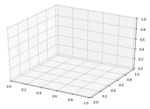

First, we imported the pyplot submodule from Matplotlib. Then, we enabled 3D plots by importing the mplot3d submodule. After that, we created the Figure (fig) object by specifying the size in inches. It acts as the canvas on which we create the plot or Axes (ax) object. Note that we haven’t added the Axis (x, y, z-axis) objects and any interactivity to the plot yet.

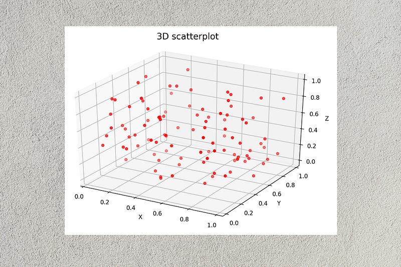
Now, we’ll add data to the empty plot and make a scatterplot by using the scatter3D method of the ax object. We’ll also add Axis (x, y, z-axis) objects to the plot. Here, we use synthetic (simulated) data generated by the NumPy random function.

import numpy as np

np.random.seed(3)
y = np.random.random(100)
x = np.random.random(100)
z = np.random.random(100)

ax.scatter3D(x, y, z, color='red')

ax.set_title("3D scatterplot", pad=25, size=15)
ax.set_xlabel("X") 
ax.set_ylabel("Y") 
ax.set_zlabel("Z")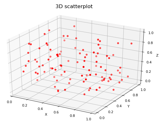

Note that we haven’t added any interactivity to the plot yet. To add interactivity, you should add %matplotlib notebook or %matplotlib qt at the beginning of the code.

%matplotlib qt
import matplotlib.pyplot as plt
...

Here is the interactive pop-up window.

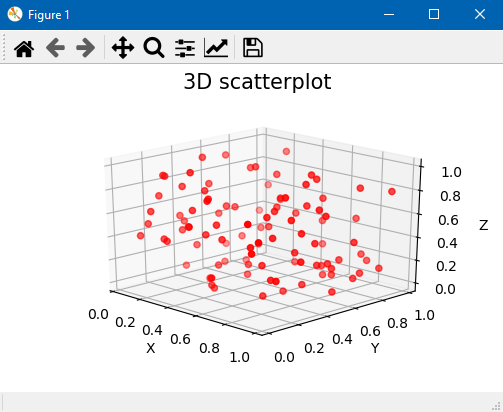
When you move the cursor over the window, the plot will rotate. You can also zoom and resize the plot by using the available tools within the window.

This is the end of today’s post.

Please let me know if you’ve any feedback.

Meanwhile, you can sign up for a membership to get full access to every story I write and I will receive a portion of your membership fee.

Thank you so much for your continuous support! See you in the next story. Happy learning to everyone!

Special credit goes to Bernard Hermant on Unsplash, who provides me with a nice cover image for this post.

Rukshan Pramoditha 2021–12–11