Creating an Innovative Pull-Back Trading Strategy.

Coding the Pull-Back Trading Strategy on the Relative Strength Index.

The Relative Strength Index is a known contrarian indicator but can also be used to confirm a new trend by other methods such as a pull-back. We are used to using this technique on the market price, but it can also be used on the technical indicators. This article discusses the method in detail.

I have just published a new book after the success of the previous book titled New Technical Indicators in Python. The new book features a more complete description and addition of strategies with a Github page dedicated to the code (being constantly populated and updated). If you feel that this interests you, do not hesitate, also, the PDF version is purchasable, you can contact me on Linkedin.

The Relative Strength Index

The RSI is without a doubt the most famous momentum indicator out there, and this is to be expected as it has many strengths especially in ranging markets. It is also bounded between 0 and 100 which makes it easier to interpret. The RSI is notably used in many ways, among them:

• The extremes strategy: Where we search for overbought an oversold levels to initiate contrarian trades. The idea is that an overbought market has a high reading on the RSI signifying too much bullish momentum and a possible correction or even a reversal may take place. Similarly, an oversold market has a low reading on the RSI signifying too much bearish momentum and a possible correction or even a reversal may take place.
• The divergence strategy: When there is an established trend, the overall direction does not move linearly with regards to magnitude and force, meaning that when a market is rising, its momentum strength is not stable. At the begining it is usually strong but by profit taking and lower convictions, the market starts to lose some strength, thus, continuing to rise but struggling to do so. This is where we see a bearish divergence on the RSI. A divergence signifies the trend’s exhaustion and may signal a correction or even a reversal. Visually, a bearish divergence is when we see the market making higher highs while the RSI is making lower highs. Similarly, a bullish divergence is when we see the market making lower lows while the RSI is making higher lows.

The fact that it is famous, contributes to the efficacy of the RSI. This is because the more traders and portfolio managers look at the indicator, the more people will react based on its signals and this in turn can push market prices. Of course, we cannot prove this idea, but it is intuitive as one of the basis of Technical Analysis is that it is self-fulfilling.

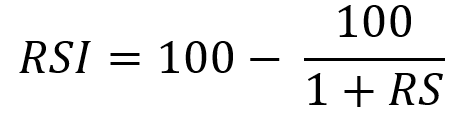
The RSI is calculated using a rather simple way. We first start by taking price differences of one period. This means that we have to subtract every closing price from the one before it. Then, we will calculate the smoothed average of the positive differences and divide it by the smoothed average of the negative differences. The last calculation gives us the Relative Strength which is then used in the RSI formula to be transformed into a measure between 0 and 100.

To calculate the Relative Strength Index through the following function, we need an OHLC array (not a data frame). This means that we will be looking at an array of 4 columns. The function for the Relative Strength Index is therefore:

def rsi(Data, lookback, close, where, width = 1, genre = 'Smoothed'):
    
    # Adding a few columns
    Data = adder(Data, 7)
    
    # Calculating Differences
    for i in range(len(Data)):
        
        Data[i, where] = Data[i, close] - Data[i - width, close]
     
    # Calculating the Up and Down absolute values
    for i in range(len(Data)):
        
        if Data[i, where] > 0:
            
            Data[i, where + 1] = Data[i, where]
            
        elif Data[i, where] < 0:
            
            Data[i, where + 2] = abs(Data[i, where])
            
    # Calculating the Smoothed Moving Average on Up and Down
    absolute values    
    if genre == 'Smoothed':                    
      lookback = (lookback * 2) - 1 # From exponential to smoothed
      Data = ema(Data, 2, lookback, where + 1, where + 3)
      Data = ema(Data, 2, lookback, where + 2, where + 4)
    
    if genre == 'Simple':                    
      Data = ma(Data, lookback, where + 1, where + 3)
      Data = ma(Data, lookback, where + 2, where + 4)
    
    # Calculating the Relative Strength
    Data[:, where + 5] = Data[:, where + 3] / Data[:, where + 4]
    
    # Calculate the Relative Strength Index
    Data[:, where + 6] = (100 - (100 / (1 + Data[:, where + 5])))  
    
    # Cleaning
    Data = deleter(Data, where, 6)
    Data = jump(Data, lookback)                        

    return Data

We need to define the primal manipulation functions first in order to use the RSI’s function on OHLC data arrays.

# The function to add a certain number of columns
def adder(Data, times):
    
    for i in range(1, times + 1):
    
        z = np.zeros((len(Data), 1), dtype = float)
        Data = np.append(Data, z, axis = 1)                

    return Data

# The function to deleter a certain number of columns
def deleter(Data, index, times):
    
    for i in range(1, times + 1):
    
        Data = np.delete(Data, index, axis = 1)               
    
    return Data

# The function to delete a certain number of rows from the beginning
def jump(Data, jump):
    
    Data = Data[jump:, ]
    
    return Data

Now, we will see a less known strategy on the RSI which is generally used as a confirmation of the new expected reversal. It can be considered as an entry technique on the extremes strategy.

If you are interested in seeing more technical indicators and back-tests, feel free to check out the below article:

Creating the Pull-Back Strategy

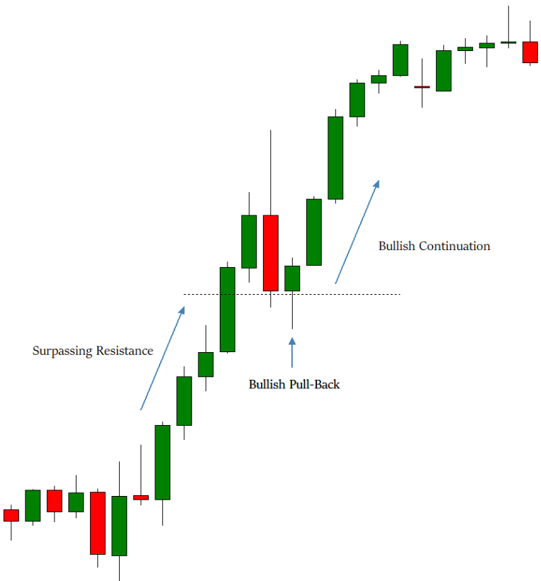
The pull-back method is a very known technique in the world of trading, it is based on the fact that after a breakout, the market will stabilize before continuing higher due to profit-taking and increased orders in the cotnrarain direction in anticipation that the support/resistance level will hold. This generally provides a good entry level for the trades in the right direction. Below is an illustration of a pull-back.

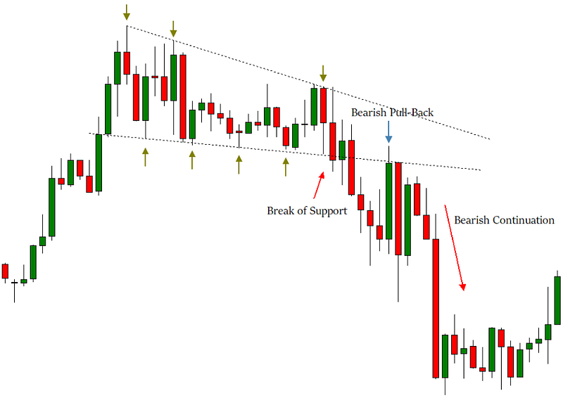
Another example can be an exit of a triangular configuration such as the below. The market has broken its descending support outlined with the green upwards pointing arrows, then tried coming back but found resistance at the same descending support line which is now resistance, to finally continue the drop. This is a perfect example of a pull-back.

The idea of the strategy is to apply this method on the famous technical indicator, the Relative Strength Index. It will be easier to code as we have objective barriers already which we call oversold and overbought levels.

• An oversold level is typically below 30 and refers to a state of the market where selling activity was a bit extreme. Therefore, whenever the RSI surpasses the 30 level after being below it, and then retraces back close to it, a bullish signal is generated.
• An overbought level is typically above 70 and refers to a state of the market where buying activity was a bit extreme. Therefore, whenever the RSI breaks the 70 level after being above it, and then retraces back close to it, a bearish signal is generated.

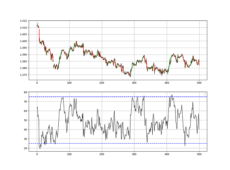
Basically, we will be applying the exact same pull-back method on the Relative Strength Index and using the signals as directional confirmation.

lookback         = 13
upper_barrier    = 70
lower_barrier    = 30
margin           = 2 

def signal(Data, rsi_column, buy, sell):
    
    Data = adder(Data, 20)
    
    for i in range(len(Data)):
            
        if Data[i, rsi_column] >= lower_barrier and Data[i, rsi_column] <= lower_barrier + margin and Data[i - 1, rsi_column] > lower_barrier and Data[i - 2, rsi_column] < lower_barrier:
            Data[i, buy] = 1
            
        elif Data[i, rsi_column] <= upper_barrier and Data[i, rsi_column] >= upper_barrier - margin and Data[i - 1, rsi_column] < upper_barrier and Data[i - 2, rsi_column] > upper_barrier:
            Data[i, sell] = -1    
            
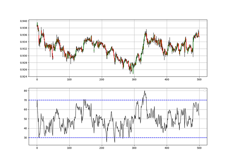
    return Data

# The margin variable is the maximum distance for the pull-back to be valid. A margin of 2 and a lower barrier of 30 means that that the RSI can retrace back to between 30 and 32 and the event can still be considered a pull-back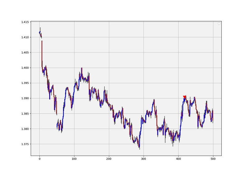

The chart above shows the one signal generated by the algorithm. It can be seen that the moment the RSI has fulfilled all the conditions, a bearish signal around the top has been generated.

Many optimization and modifications can be added to the algorithm such as:

• Tweaking the margin variable so that more pull-backs are taken into account. We should not make this variable too high so that we remain in the spirit of the strategy.
• Adding the condition that looks more into the past so that slow pull-backs are considered.
• Tweaking the RSI’s lookback period even though the default values are recommended as a very short RSI has unreliable pull-back signals due to the short life between the extremes.
• Adding a moving average break confirmation signal.

The pull-back method is theoretically a laggard compared to the extremes and the barrier exit ones but is the best regarding to entry optimization and realization of the reaction due to the fact that the extremes can last a long time and the barrier exit can provide an expensive entry level. Also, the pull-back method can help avoid false breakouts.

If you are interested by market sentiment and how to model the positioning of institutional traders, feel free to have a look at the below article:

The Framework of Strategy Back-testing

Having had the signals, we now know when the algorithm would have placed its buy and sell orders, meaning, that we have an approximate replica of the past where can can control our decisions with no hindsight bias. We have to simulate how the strategy would have done given our conditions. This means that we need to calculate the returns and analyze the performance metrics. This section will try to cover the essentials and provide a framework. We can first start with the simplest measure of all, the profit and loss statement. When we back-test our system, we want to see whether it has made money or lost money. After all, it is a game of wealth. This can be done by calculating the gains and losses, the gross and net return, as well as charting the equity plot which is simply the time series of our balance given a perfect algorithm that initiates buy and sell orders based on the strategy. Before we see that, we have to make sure of the following since we want a framework that fits everywhere:

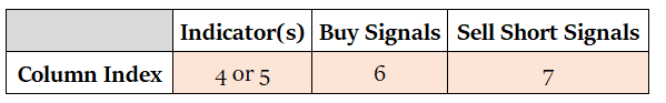
The above table says that we need to have the indicator or the signal generator at column 4 or 5 (Remember, indexing at Python starts at zero). The buy signal (constant = 1) at the column indexed at 6, and the sell short signal (constant = -1) at the column indexed at 7. This ensures the remainder of the code below works how it should work. The reason for this is that on an OHLC data, we have already the first 4 columns occupied, leaving us 1 or 2 columns to place our Indicators, before having two signal columns. Using the deleter function seen above can help you achieve this order in case the indicators occupy more than 2 columns.

The first step into building the Equity Curve is to calculate the profits and losses from the individual trades we are taking. For simplicity reasons, we can consider buying and selling at closing prices. This means that when we get the signal from the indicator or the pattern on close, we initiate the trade on the close until getting another signal where we exit and initiate the new trade. In real life, we do this mainly on the next open, but generally in FX, there is not a huge difference. The code to be defined for the profit/loss columns is the below:

def holding(Data, buy, sell, buy_return, sell_return):for i in range(len(Data)):
        try:
            if Data[i, buy] == 1: 
               for a in range(i + 1, i + 1000):                        
                  if Data[a, buy] != 0 or Data[a, sell] != 0:
                     Data[a, buy_return] = (Data[a, 3] - Data[i, 3])
                        break                        
                    else:
                        continue
                
            elif Data[i, sell] == -1:        
               for a in range(i + 1, i + 1000):                        
                  if Data[a, buy] != 0 or Data[a, sell] != 0:
                    Data[a, sell_return] = (Data[i, 3] - Data[a, 3])
                        break                                        
                    else:
                        continue                                         
        except IndexError:
            pass

# Using the function
holding(my_data, 6, 7, 8, 9)

This will give us columns 8 and 9 populated with the gross profit and loss results from the trades taken. Now, we have to transform them into cumulative numbers so that we calculate the Equity Curve. To do that, we use the below indexer function:

def indexer(Data, expected_cost, lot, investment):
    
    # Charting portfolio evolution  
    indexer = Data[:, 8:10]    
    
    # Creating a combined array for long and short returns
    z = np.zeros((len(Data), 1), dtype = float)
    indexer = np.append(indexer, z, axis = 1)
    
    # Combining Returns
    for i in range(len(indexer)):
        try:    
          if indexer[i, 0] != 0:
             indexer[i, 2] = indexer[i, 0] - (expected_cost / lot)
                
          if indexer[i, 1] != 0:
             indexer[i, 2] = indexer[i, 1] - (expected_cost / lot)
        except IndexError:
            pass
        
    # Switching to monetary values
    indexer[:, 2] = indexer[:, 2] * lot
    
    # Creating a portfolio balance array
    indexer = np.append(indexer, z, axis = 1)
    indexer[:, 3] = investment 
    
    # Adding returns to the balance    
    for i in range(len(indexer)):
    
        indexer[i, 3] = indexer[i - 1, 3] + (indexer[i, 2])
    
    indexer = np.array(indexer)
    
    return np.array(indexer)

# Using the function for a 0.1 lot strategy on $10,000 investment
expected_cost = 0.5 * (lot / 10000) # 0.5 pip spread
investment    = 10000                  
lot           = 10000
equity_curve = indexer(my_data, expected_cost, lot, investment)

The below code is used to generate the chart. Note that the indexer function nets the returns using the estimated transaction cost, hence, the equity curve that would be charted is theoretically net of fees.

plt.plot(equity_curve[:, 3], linewidth = 1, label = 'EURUSD)
plt.grid()
plt.legend()
plt.axhline(y = investment, color = 'black’, linewidth = 1)
plt.title(’Strategy’, fontsize = 20)

Now, it is time to start evaluating the performance using other measures.

I will present quickly the main ratios and metrics before presenting a full performance function that outputs them all together. Hence, the below discussions are mainly informational, if you are interested by the code, you can find it at the end.

Hit ratio       =  42.28 % # Simulated Ratio

The Hit Ratio is extremely easy to use. It is simply the number of winning trades over the number of the trades taken in total. For example, if we have 1359 trades over the course of 5 years and we have been profitable in 711 of them , then our hit ratio (accuracy) is 711/1359 = 52.31%.

The Net Profit is simply the last value in the Equity Curve net of fees minus the initial balance. It is simply the added value on the amount we have invested in the beginning.

Net profit      =  $ 1209.4 # Simulated Profit

The net return measure is your return on your investment or equity. If you started with $1000 and at the end of the year, your balance shows $1300, then you would have made a healthy 30%.

Net Return      =  30.01% # Simulated Return

A quick glance on the Average Gain across the trades and the Average Loss can help us manage our risks better. For example, if our average gain is $1.20 and our average loss is $4.02, then we know that something is not right as we are risking way too much money for way too little gain.

Average Gain    =  $ 56.95 per trade # Simulated Average Gain
Average Loss    =  $ -41.14 per trade # Simulated Average Loss

Following that, we can calculate two measures:

• The theoretical risk-reward ratio: This is the desired ratio of average gains to average losses. A ratio of 2.0 means we are targeting twice as much as we are risking.
• The realized risk-reward ratio: This is the actual ratio of average gains to average losses. A ratio of 0.75 means we are targeting three quarters of what we are risking.

Theoretical Risk Reward = 2.00 # Simulated Ratio
Realized Risk Reward    = 0.75 # Simulated Ratio

The Profit Factor is a relatively quick and straightforward method to compute the profitability of the strategy. It is calculated as the total gross profit over the total gross loss in absolute values, hence, the interpretation of the profit factor (also referred to as the profitability index in the jargon of corporate finance) is how much profit is generated per $1 of loss. The formula for the profit factor is:

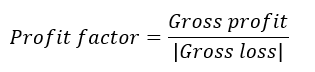
Profit factor   =  1.34 # Simulated Profit Factor

Expectancy is a flexible measure presented by the well-known Laurent Bernut that is composed of the average win/loss and the hit ratio. It provides the expected profit or loss on a dollar figure weighted by the hit ratio. The win rate is what we refer to as the hit ratio in the below formula, and through that, the loss ratio is 1 — hit ratio.

Expectancy      =  $ 1.33 per trade # Simulated Expectancy

Another interesting measure is the number of trades. This is simply to understand the frequency of the trades we have.

Trades          = 3697 # Simulated Number

Now, we are ready to have all of the above metrics shown at the same time. After calculating the indexer function, we can use the below performance function to give us the metrics we need:

def performance(indexer, Data, name):
    
    # Profitability index
    indexer = np.delete(indexer, 0, axis = 1)
    indexer = np.delete(indexer, 0, axis = 1)
    
    profits = []
    losses  = []
    np.count_nonzero(Data[:, 7])
    np.count_nonzero(Data[:, 8])
    
    for i in range(len(indexer)):
        
        if indexer[i, 0] > 0:
            value    = indexer[i, 0]
            profits  = np.append(profits, value)
            
        if indexer[i, 0] < 0:
            value    = indexer[i, 0]
            losses   = np.append(losses, value)
    
    # Hit ratio calculation
    hit_ratio = round((len(profits) / (len(profits) + len(losses))) * 100, 2)
    
    realized_risk_reward = round(abs(profits.mean() / losses.mean()), 2)
    
    # Expected and total profits / losses
    expected_profits = np.mean(profits)
    expected_losses  = np.abs(np.mean(losses))
    total_profits    = round(np.sum(profits), 3)
    total_losses     = round(np.abs(np.sum(losses)), 3)
    
    # Expectancy
    expectancy    = round((expected_profits * (hit_ratio / 100)) \
                   - (expected_losses * (1 - (hit_ratio / 100))), 2)
        
    # Largest Win and Largest Loss
    largest_win = round(max(profits), 2)
    largest_loss = round(min(losses), 2)        

    # Total Return
    indexer = Data[:, 10:12]    
    
    # Creating a combined array for long and short returns
    z = np.zeros((len(Data), 1), dtype = float)
    indexer = np.append(indexer, z, axis = 1)
    
    # Combining Returns
    for i in range(len(indexer)):
        try:    
          if indexer[i, 0] != 0:
             indexer[i, 2] = indexer[i, 0] - (expected_cost / lot)
                
          if indexer[i, 1] != 0:
             indexer[i, 2] = indexer[i, 1] - (expected_cost / lot)
        except IndexError:
            pass
        
    # Switching to monetary values
    indexer[:, 2] = indexer[:, 2] * lot
    
    # Creating a portfolio balance array
    indexer = np.append(indexer, z, axis = 1)
    indexer[:, 3] = investment 
    
    # Adding returns to the balance    
    for i in range(len(indexer)):
    
        indexer[i, 3] = indexer[i - 1, 3] + (indexer[i, 2])
    
    indexer = np.array(indexer)
    
    total_return = (indexer[-1, 3] / indexer[0, 3]) - 1
    total_return = total_return * 100
    
    
    print('-----------Performance-----------', name)
    print('Hit ratio       = ', hit_ratio, '%')
    print('Net profit      = ', '$', round(indexer[-1, 3] - indexer[0, 3], 2))
    print('Expectancy      = ', '$', expectancy, 'per trade')
    print('Profit factor   = ' , round(total_profits / total_losses, 2)) 
    print('Total Return    = ', round(total_return, 2), '%')
    print('')    
    print('Average Gain    = ', '$', round((expected_profits), 2), 'per trade')
    print('Average Loss    = ', '$', round((expected_losses * -1), 2), 'per trade')
    print('Largest Gain    = ', '$', largest_win)
    print('Largest Loss    = ', '$', largest_loss)    
    print('')
    print('Realized RR     = ', realized_risk_reward)
    print('Minimum         =', '$', round(min(indexer[:, 3]), 2))
    print('Maximum         =', '$', round(max(indexer[:, 3]), 2))
    print('Trades          =', len(profits) + len(losses))

# Using the function
performance(equity_curve, my_data, 'EURUSD)

This should give us something like the below:

-----------Performance----------- EURUSD
Hit ratio       =  42.28 %
Net profit      =  $ 1209.4
Expectancy      =  $ 0.33 per trade
Profit factor   =  1.01
Total Return    =  120.94 %
Average Gain    =  $ 56.95 per trade
Average Loss    =  $ -41.14 per trade
Largest Gain    =  $ 347.5
Largest Loss    =  $ -311.6Realized RR     =  1.38
Minimum         = $ -1957.6
Maximum         = $ 4004.2
Trades          = 3697

# All of the above are simulated results and do not reflect the presented strategy or indicator

Conclusion & Important Disclaimer

Remember to always do your back-tests. You should always believe that other people are wrong. My indicators and style of trading may work for me but maybe not for you.

I am a firm believer of not spoon-feeding. I have learnt by doing and not by copying. You should get the idea, the function, the intuition, the conditions of the strategy, and then elaborate (an even better) one yourself so that you back-test and improve it before deciding to take it live or to eliminate it. My choice of not providing Back-testing results should lead the reader to explore more herself the strategy and work on it more. That way you can share with me your better strategy and we will get rich together.

To sum up, are the strategies I provide realistic? Yes, but only by optimizing the environment (robust algorithm, low costs, honest broker, proper risk management, and order management). Are the strategies provided only for the sole use of trading? No, it is to stimulate brainstorming and getting more trading ideas as we are all sick of hearing about an oversold RSI as a reason to go short or a resistance being surpassed as a reason to go long. I am trying to introduce a new field called Objective Technical Analysis where we use hard data to judge our techniques rather than rely on outdated classical methods.

If you are also interested by more technical indicators and using Python to create strategies, then my best-selling book on Technical Indicators may interest you: