Creating a New Stochastic Volatility Model from Scratch (Part 3 of 3)

Creation of a new stochastic volatility model for volatility clustering using Bitcoin Price data

Introduction

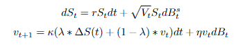
The term ‘stochastic’ is defined as randomness stemming from an underlying probability distribution. Stochastic volatility models have a component wherein variance is randomly distributed. By leveraging the fact that price movements are stochastic, we can introduce a function that itself is inherently stochastic. The equation below is based on geometric Brownian motion where ‘v’ is no longer constant, varying in time.

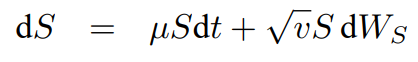
The main focus for stochastic volatility models is the variable, ‘v,’ which is not constant throughout time.

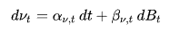
The change in v is given as two new functions, expressed in terms of v: Alpha captures trends in (v) and Beta captures the randomness.

A more comprehensive introduction is given in Part 1, where I explained how to create a new Stochastic Volatility model from scratch.

Creating a New Stochastic Volatility Model from Scratch (Part 1 of 3) — Medium

Creation of an Innovative Stochastic Model

The goal of this section is to demonstrate how we can start from a general mathematical framework for stochastic volatility modeling and introduce equations to fit the needs of our application. In this case our application is to capture the fact that volatility clusters.

Recall that the general framework for the creation of a stochastic volatility model is given as:

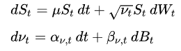
We will model both Alpha and Beta as functions of v. Note that it is important to consider the correlation structure between W(t) and B(t). One key concept that I would like my volatility model to capture is the clustering of price changes. The Alpha function will be responsible for capturing the clustering of price changes.

Recall that in the Heston model (see part 2 for more details) a constant, k, dictates how fast the volatility mean reverts. Going forward, we will build upon this concept and create a more sophisticated approach.

I want to be able to dictate the decay of volatility clustering exponentially. This new formulation is controlled by a constant value lambda (λ ∗ ∆S(t) + (1 − λ) ∗ v). The part of this equation responsible for representing the volatility clustering is ((1 − λ) ∗ v).

Lambda becomes a balancing parameter between the current change in price and the previous volatility.

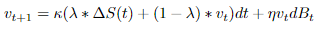
The ∆S(t) is the change in the asset price at time, t. Vt is the modelled volatility; n is a constant that controls the stochastic part of the model, and dBt is a Wiener process that is covariant with the randomness of the price changes of the asset.

• dBt is a Wiener process that is covariant with the randomness of the price changes of the asset
• ∆S(t) is the change in price
• Vt is the volatility of the asset price
• n is a constant that controls the stochastic part of the model
• λ is the control on the long-term price variance
• dt is the indefinitely small positive time increment

Lambda can be fit with using a data driven approach with an error minimization formula.

Simulating the Innovative Stochastic Model in Python

The new model is still stochastic in nature, where both the price changes and volatility are simulated as random changes.

The above equations model forward both the asset price S and the volatility (V). In the first equation, r is responsible for how the current price information is used for the next price.

• Paths represents the number of simulations
• Steps is the length of each simulation
• V0 is the starting volatility
• S is the starting price

The Price paths are randomly simulated, here we have a good mix of low and high volatility over the time period.

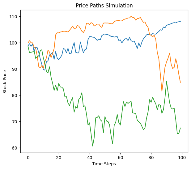
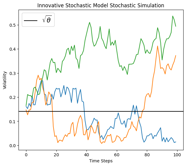
The Simulated prices demonstrate both low volatility (Blue), medium volatility (Orange) and high volatility (Green). Below is the modelled volatility using the innovate model. Strong price moves are reciprocated by higher volatility so our model is demonstrating promise.

Testing the innovative model in terms of predictability for future volatility is measured using RMSE.

Testing Innovative Volatility Model using Bitcoin price data

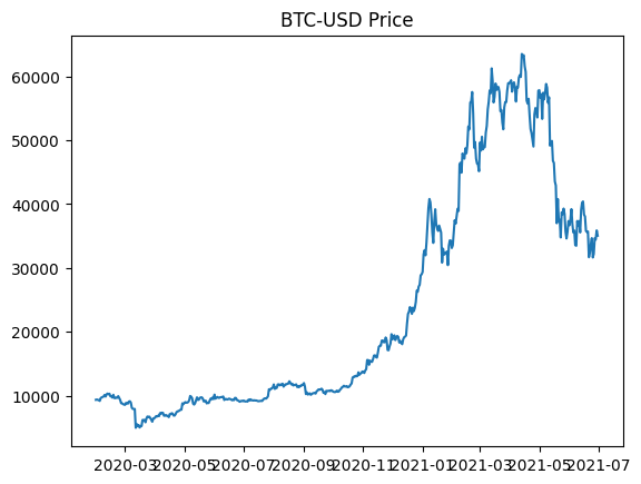
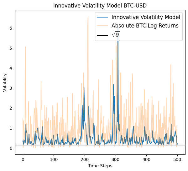
The data used will be the price change of bitcoin (BTC-USD) over the last year, on the daily time scale. The data for this investigation is obtained using Yahoo BTC-USD data from the yfinance API. The testing period contains both sections of prolonged low volatility and high volatility which will test volatility clustering.

Let’s now delve into an application of the innovate stochastic model to simulate the volatility of the BTC-USD price in Python. When using real data, we need to define the correlation between the two Weiner processes shown below:

If you want to know more about decomposition and stationary time series, you can read my comprehensive guide to modelling the volatility of top cryptocurrency coins.

For this application, the model parameters (Lambda, Kappa, xi) are set manually. However, their optimal values can be found using a grid search or loss function, depending on the application.

The price change is measured as the log of the fractional change. One of the effects of the model structure is the fast decay of volatility, which is controlled by Lambda.

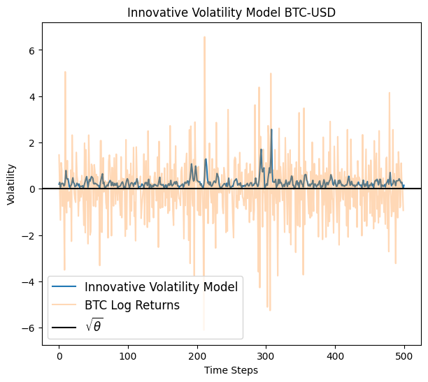
Here, the modelled volatility is mean reverting, meaning that the price returns to a mean value. Moreover, the modelled volatility is dynamic to capturing increases and decreases to the volatility. The non-constant volatility model is superior to the constant volatility by capturing clusters and changes in the underlying asset price.

I want to further examine the change in the modelled volatility by adjusting the parameters. The effect of increasing Xi increases the numerical value for the modelled volatility.

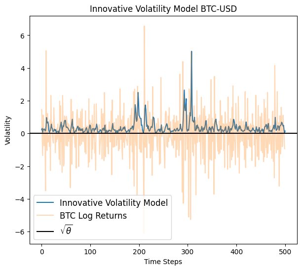
Keep in mind that this model predicts the “one day ahead” forecast. There are other methods to lengthen the forecast and predict several days into the future, however as they are tangential to the main topic, I don’t touch upon those methods in this article.

Conclusion

The purpose of this article was to demonstrate stochastic volatility modeling. Hopefully you are left with a few takeaways about creating a volatility model from a mathematical framework. The advantage of the new model is that it takes into account volatility clustering and a fast decay back to the mean.

About the author:

Ethan Skinner holds a Master of Applied Mathematics from Ryerson University, in Toronto, Canada, where he also completed his Bachelor’s in Aerospace Engineering. Ethan has published two academic papers at the IEEE COMSAC 2021 conference.

He was part of the financial mathematics group specializing in statistics and studied volatility modelling and algorithmic trading in-depth. Ethan previously worked as an engineering professional at Bombardier Aerospace, where he was responsible for modelling the life-cycle costs associated with aircraft maintenance.

I am actively training for triathlon and love fitness.

If you have any suggestions on the topics below let me know

• Data science
• Machine Learning
• Mathematics
• Statistical Modelling

Linkedin: https://www.linkedin.com/in/ethanjohnsonskinner/

Twitter: @Ethan_JS94

Subscribe to DDIntel Here.

Visit our website here: https://www.datadriveninvestor.com

Join our network here: https://datadriveninvestor.com/collaborate