Creating a New Stochastic Volatility Model from Scratch (Part 1 of 3)

Introduction to stochastic volatility models (GARCH) and the creation of a new stochastic volatility model for volatility clustering using Bitcoin Price data

Introduction

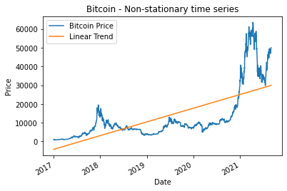
Why do we model volatility in financial markets? There exists a simple principle that changes in price movements are clustered together. Large changes in the price of an asset are often followed by other large changes and small changes are accordingly often followed by other small changes.

Moreover, these seemingly random price changes are stochastic in nature. A Stochastic process is defined as a random process. In the financial markets this can be observed as the price movements of an asset.

The Wiener process (Brownian Motion) is the process that is used to model financial markets. Mathematically the Wiener process is defined as W(t) where W(0) = 0 and W(t)-W(s) is a gaussian with N(0,σ).

Each change in the random process is independent. When each change is randomly modeled with a gaussian process with zero mean, the expectation is also zero. Because this is not reflective of a financial market, we introduce drift. Here, drift is defined as a general upward or downward movement in price over time.

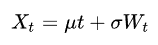
Extending the Wiener process with the inclusion of drift, we define the standard model for geometric Brownian motion. Here, drift is the term, μt, and the price movement is X(t).

The stochastic differential equation with constant volatility is defined as:

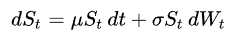
W(t) is a Wiener process, S(t) is the asset price and sigma is the constant volatility.

Historically, in financial markets, volatility has never been constant over time; stochastic volatility models overcome this limitation by varying throughout time.

Introduction to the basics of volatility modelling

To understand the volatility of future returns, we must first define the volatility mathematically so we can build our model.

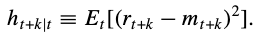
Interpreting future volatility at k steps ahead, let’s first observe how we can build up volatility.

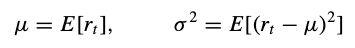
We have the mean and variance of a given time series. In our case, rᵗ represents the log returns for a given asset. E is defined as the expectation or expected value.

The expectation is simply the weighted mean — or in mathematical terms, the first moment. The variance then becomes the second moment. I will rewrite the variance formula to make it clear why we call this the second moment.

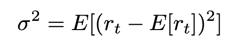
The above expression contains within it the expectation of the expectation, and is called the second moment in statistics. Mathematically, the interpretation of the formula above is: expectation of the difference between the daily log returns and the expectation of all the log returns. In simple terms, the formula is a measure between the daily return and average return.

Using the same framework for the standard deviation we can now look at how the volatility of future returns is formulated.

Let t be the current day and k be some number of future time steps. The above formula is the same as the variance formula with one key difference: future volatility is conditional on the current time step, t. The statement [ht+k|t] says that future volatility is conditional (dependent) on the current volatility. This ties into volatility clustering — the idea that volatility shocks today will influence the expectation of volatility many periods in the future.

With the goal clearly defined we can now define some key principles that we want our volatility forecasting model to consider.

• Volatility is mean reverting (high volatile periods are followed by low volatile periods)
• Future volatility is dependent on the current volatility (Volatility Clustering)
• External variables impact volatility (Company Quarterly reports, Economical data, employment data and inflation reports)

Stochastic Volatility Models

“Stochastic” is defined as randomness stemming from an underlying probability distribution. Stochastic volatility models have a component where the variance is randomly distributed. By using the idea that price movements are stochastic we can introduce a function that itself is inherently stochastic. The equation below is based on geometric Brownian motion where v is not constant and varies in time.

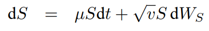
Since this is the starting point for constant volatility models I will break it down. The three main components are as follows, the change in price is equal to general up/down trend plus some random behavior.

The change in price (S) equals drift multiplied by the Asset price at time (t) multiplied by the change in time plus v(t) (function that models the volatility of S(t)) multiplied by asset price at time (t) multiplied by a standard Wiener process (random).

The main focus for stochastic volatility models is to model variable (v) which is not constant throughout time.

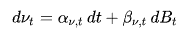
The change in (v) is given as two new functions in terms of (v). Where alpha capture trends in (v) and beta captures the randomness.

Using this stochastic volatility framework will be key in the creation of the innovative volatility model

GARCH Model

The GARCH model is one of the most common volatility models. The Generalized Autoregressive Conditional Heteroscedastic (GARCH) model is given as:

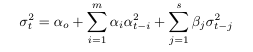
The GARCH model is an expansion on the ARCH model. In the ARCH(q) process the conditional variance is specified as a linear function of past sample variances only, whereas the GARCH(p, q) process accounts for lagged conditional variances as well.

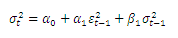
The GARCH(1,1) model is given as

Below is the implementation of the GARCH model in Python using BTC as the sample data.

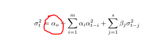
Looking back at the GARCH formula the (alpha0) term dictates the mean to which the volatility reverts to.

GARCH Implementation in Python

The implementation in Python for the GARCH model is shown below. In line 20 we are able to control the number of terms for the GARCH model, the defaults are p = 1 & q = 1.

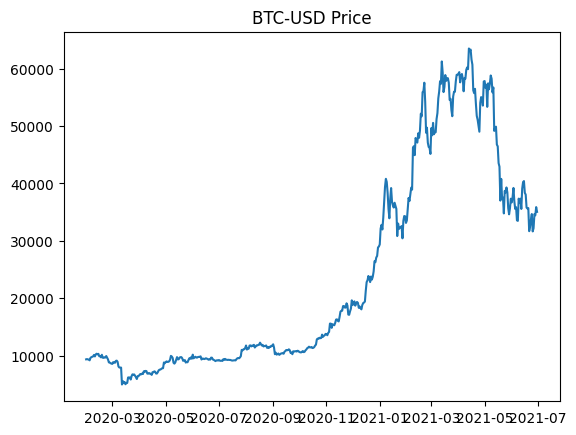
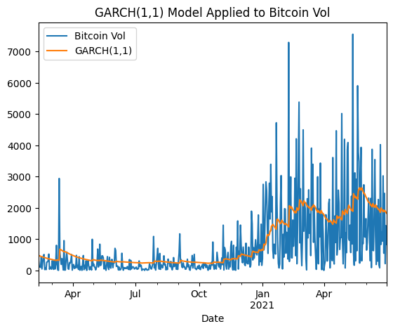
Using the price change of bitcoin over the last year on the daily time scale. The data for this investigation is fetched using yahoo BTC-USD data from the yfinance API. The testing period contains both sections of prolonged low volatility and high volatility which will be good when testing the various models.

Plotting the bitcoin volatility (price changes) with the modelled GARCH volatility. The modelled volatility displays mean reverting characteristic where large price changes cause upward spikes and then decay back down towards the mean volatility.

Constant Mean - GARCH Model Results                       ====================================================================Dep. Variable:                  Close   R-squared:                       0.000 Mean Model:             Constant Mean   Adj. R-squared:                  0.000 Vol Model:                      GARCH   Log-Likelihood:               -7205.30 Distribution:                  Normal   AIC:                           14418.6 Method:            Maximum Likelihood   BIC:                           14437.7                                         No. Observations:                  881 Date:                Mon, Sep 26 20xx   Df Residuals:                      880 Time:                        xx:xx:xx   Df Model:                            1                                  Mean Model                                  ====================================================================     coef    std err          t      P>|t|      95.0% Conf. Int. ---------------------------------------------------------------------------- mu           280.6952     33.780      8.310  9.609e-17                               Volatility Model                               ====================================================================         coef    std err          t      P>|t|       95.0% Conf. Int. ---------------------------------------------------------------------------omega        844.5496    729.040      1.158      0.247 
alpha[1]       0.0438  1.157e-02      3.788  1.520e-04  
beta[1]        0.9562  1.250e-02     76.476      0.000      ====================================================================

The output for the GARCH modelling process provides a plethora of information. Let’s begin with the coefficients for our GARCH(1,1) model. Beta is representative of the moving average and controls how the previous volatility impacts the current. When beta > 1 the variance grows to infinity and when beta < 1 it decays with time. Omega is the standard deviation for returns; we are on a daily scale which explains why omega is so high. The alpha term tells us how much the previous period’s volatility to carry forward to today.

The input into the GARCH model is the absolute value of the daily price change.

Conclusion

This was part one of three introducing stochastic volatility modeling. In the next part, I will expand on the Heston model, and then finally move to an innovative volatility model. Hopefully you have a few takeaways about how the GARCH model works and its benefits. In the next section, I will introduce Heston’s model and explore how we can use it to model BTC-USD price volatility.

About the author:

Ethan Skinner holds a Master’s of Applied Mathematics from Ryerson University, in Toronto, Canada, where he also completed his Bachelor’s in Aerospace Engineering. Ethan has published two academic papers at the IEEE COMSAC 2021 conference.

He was part of the financial mathematics group specializing in statistics, and studied volatility modelling and algorithmic trading in-depth. Ethan previously worked as an engineering professional at Bombardier Aerospace, where he was responsible for modelling the life-cycle costs associated with aircraft maintenance.

I am actively training for triathlon and love fitness.

If you have any suggestions on the topics below let me know

• Data science
• Machine Learning
• Mathematics
• Statistical Modelling

LinkedIn: https://www.linkedin.com/in/ethanjohnsonskinner/

Twitter : @Ethan_JS94

Subscribe to DDIntel Here.

Join our network here: https://datadriveninvestor.com/collaborate