A Baby Robot’s guide to Reinforcement Learning

Creating a Custom Gym Environment for Jupyter Notebooks

Part 2: Rendering to Jupyter Notebook Cells

Updated 7th January 2023:

Development of the Open AI Gym library for Reinforcement Learning, which is the base framework originally described in this article, has stopped. It has now been replaced by Gymnasium, a new package managed by the Farama Foundation.

In most cases this new framework remains the same as the original, but there have been a few subtle changes to the API. Consequently this article and its accompanying code samples have been updated to take account of these changes and to make use of this latest framework.

Therefore, although the framework is still referred to as ‘Gym’, this actually means the new ‘Gymnasium’ version of the library.

Introduction

In Part One, we saw how a custom Gym environment for Reinforcement Learning (RL) problems could be created, simply by extending the Gym base class and implementing a few functions. However, the custom environment we ended up with was a bit basic, with only a simple text output.

So, in this part, we’ll extend this simple environment by adding graphical rendering. Additionally, this rendered output will be explicitly targeted at Jupyter Notebooks, producing a graphical representation of the environment directly into the notebook cells.

All of the related code for this article can be found on Github. Additionally, the custom Baby Robot Gym Environment that we create can be installed by running ‘pip install babyrobot’ and you can play with this in the accompanying API notebook.

Also, an interactive version of this article can be found in notebook form, where you can actually run all of the code snippets described below.

Introduction to the ipycanvas Library

When running a Reinforcement Learning problem in a Jupyter Notebook, it’s very easy to write text into the notebook cell to show how things are progressing. However, given the large amount of information that can be generated over time, a much clearer representation can be obtained by creating a graphical view of the environment.

Quite often this graphical view is generated by taking snapshot images of the environment at each time-step and then joining these together, at the end of the episode, to create a short movie. This can then be played back within the notebook to see how things progressed.

The downside with this approach is that you need to wait for the movie to be created. Ideally we want to see the changes that occur in our environment happening in real time. We need something that can be added to a notebook cell, then drawn to and updated as actions take place.

This exact functionality can be achieved using the HTML canvas element, which can be accessed within a Jupyter Notebook using the excellent ipycanvas library.

Example:

The first thing we’re going to need to create our Baby Robot Grid World, is the actual “world”, where all the action takes place. At its most basic, this is just a coloured rectangle. This can be created really easily in ipycanvas by simply defining a canvas and then specifying the size and colour of rectangle to draw:

In the code above, we’ve imported the ipycanvas library, then defined the dimensions of the grid world that we’re going to create. This will be a 3x3 grid, where each cell is a square of 64-pixels. Using these dimensions we can then create our canvas.

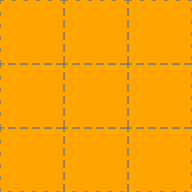
Initially the canvas will be blank, so to actually see the canvas we need to draw something. In the ‘draw_base’ function, shown above, the fill colour is set to be orange and then this is used to draw a rectangle covering the complete canvas area.

After calling this function, the final line, ‘canvas’, just draws the completed canvas into the notebook cell, as shown in Figure 1 below. This square will act as the base of our grid-world. Pretty exciting!

Adding a Grid

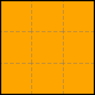
The next thing that any self-respecting Grid World is going to need is an actual grid. Again this can be easily achieved in ipycanvas by drawing a few dashed lines:

Here we’ve defined a function that sets up the canvas properties to draw a 1 pixel wide, dashed, grey line. Then we simply draw a rectangle for each cell in the grid, which gives us the output shown in Figure 2:

Adding a Border

We can improve the look of our grid world by adding a border around the outside. This is simply a black rectangle, with slightly thicker lines than the grid, and is defined in the ‘draw_border’ function. This produces the output shown below:

Adding an Animated Image

The final thing that our Baby Robot Grid World is going to need is a Baby Robot, and preferably one that moves! Since we want our robot to move over the top of the grid level, without damaging anything we’ve already drawn, we’ll use a separate canvas for our robot animation.

This is easily achieved using the MultiCanvas element. With this we can stack as many canvases as we want, and draw to each one separately, to build up our complete environment. This is shown below, where we’ve defined the MultiCanvas to have 2 layers and then used the functions from above to recreate the grid world on the first of these layers (layer index zero).

Finally, we can load in our Baby Robot image and create a very simple animation, drawing our animation onto the upper canvas (index = 1).

To make Baby Robot move across the screen we use a simple loop that clears the previous image before drawing the next one. Since there’s some padding on the image we can simply clear the area where we want to draw the new image. Both of these operations are tied together using ‘hold_canvas’ which makes things slightly smoother (for more advanced animations check out the ipycanvas documentation).

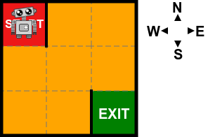
The final Baby Robot Grid World is shown in Figure 4, below:

Creating a Graphical Grid Level

Using the ipycanvas library, and the basic drawing routines described above, we can create classes that encapsulate all of the functionality required to draw a graphical grid level for our custom Gym environment.

As part of this, we have two main classes:

• GridLevel: to manage the drawing and querying of the grid level.
• RobotDraw: to draw Baby Robot onto the grid at a particular location and to do the animation as he moves between cells.

The full code for both of these classes can be found on Github.

In the code below we import these two classes and then use them to draw a default 3x3 grid level, onto which we add Baby Robot, positioned at cell [1,1].

The output we get in our Jupyter Notebook cell is shown in Figure 5 below. This gives us a default Baby Robot grid world level that we can use to create a graphical rendering function for our Gym environment.

Create a graphical Gym render function

At the end of the first part of this series on creating a custom Gym environment we’d ended up with a render function that produced this:

While providing all the important information about the current state of the environment, it’s not very exciting. Additionally, it’s a lot harder to visualise how the episode progressed. By looking at the coordinates at each time step you can sort of imagine how Baby Robot moved through the grid, but things would be much clearer if we could actually see this happening.

As we’ve seen, real time graphics can be created in a Jupyter Notebook cell using ipycanvas, so we can replace the current text-base render function with one that shows a graphical view of the environment and update this as changes occur. This is shown below:

As we’ve done previously, the new class inherits from the previous version of the environment (in this case from BabyRobotEnv_v2), which gives us all the functionality of the Gym base class, plus the extra stuff we added in the previous iterations. We then just need to provide new versions of the functions we want to replace, which in this case are as follows:

• __init__ : contains the instances of our ‘GridLevel’ and ‘RobotDraw’ classes that we need for drawing the grid and Baby Robot respectively.
• reset : puts both Baby Robot and the environment back to the initial position.
• render : moves Baby Robot to the new position (where the position has been calculated in the Gym interface’s ‘step’ function, defined in BabyRobotEnv_v2) and draws the level. This will animate the movement as Baby Robot moves from one cell to the next.

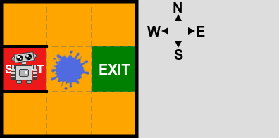
Now when we create an instance of this environment and call it’s render function, we see this:

Even better, when we run our standard reinforcement learning loop, shown above, we now get to see Baby Robot moving around the environment. Baby Robot is currently taking randomly sampled actions in his quest to find the exit, so each episode will follow a different path. One such episode is shown in Figure 7:

State specific action spaces

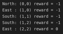
If you take a look again at the BabyRobotEnv_v3 ‘render’ function, you’ll see that we’re still printing the action, position and reward for each time step. So, in addition to the new graphical output, we’re still getting the text output from version 2 of our environment. Additionally, if you examine this text output, you’ll see entries such as the first line in Figure 5:

“North: (0,0) reward = -1”

In other words, Baby Robot was in the initial start square (0,0) and then chose to move North, which would take him straight into a wall!

Although he’s only a baby, he’s not stupid, so should only choose actions that are valid. We can achieve this by introducing a state specific action space where, rather than simply choosing from all of the actions, the action that is returned depends on the current state.

In the code above we’ve created a custom Gym Space. We’ll use this to store the actions available in the current state and then, when ‘sample’ is called, we’ll randomly select one of these actions.

Using this class we can enhance our previous environment so that, when a new state is entered, it sets up the possible actions for that state. This is shown below:

As before, we inherit from the previous environment (in this case BabyRobotEnv_v3), so that we can build on its functionality. We then add an instance of the ‘Dynamic’ class and, each time the ‘take_action’ function is called, we populate this with the actions available for the current state.

As a result, when an action is sampled for a particular state, it will be drawn from the set of valid actions, that don’t result in Baby Robot walking into a wall.

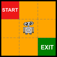
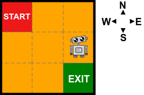
For example, for the start state, calling BabyRobotEnv_v4’s ‘show_available_actions’ function returns the actions South and East. Similarly, for grid position (2,1), shown in Figure 8, the available actions are North, South or West.

Registering and checking a local environment class

To check that our new environment conforms to the Gym API standard we can use the Gymnasium ‘check_env’ function. If this returns no warnings then we’re all good.

However, to supply our environment to this function, we first need to call ‘gym.make’ to make the environment, but before we can do this we need to have registered the environment for Gymnasium to know about it.

In the first part of this article we saw how to do this when the custom environment was contained in its own python file. In this case the ‘entry_point’ supplied to the ‘_register_’ function defines the file and class name.

Registering a local class is slightly different. In this case the ‘entry_point’ is just the class name rather than a string. So, in this case, we can register and check the BabyRobotEnv_v4 class as follows:

Enhancing the graphical environment

While it’s useful to be able to see the text output, giving the details for each action, it’s not very nice that it generates an ever increasing list of text, which eventually swamps the notebook cell.

Rather than using a print statement in the ‘render’ function we can instead write text directly to the canvas. To do this, we first need to expand the canvas to create a region where the text can be shown. By making use of the ‘__init__’ function’s ‘kwargs’ argument, we can supply an object that defines this text region:

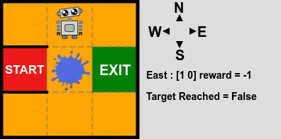
In the example above we’ve specified that we’d like a grey side panel with a width approximately equal to the width of the grid level. This then gives the following output:

All we need now is a way to write to this panel, and display the required information, each time ‘render’ is called. The next iteration of our environment contains the ‘show_info’ function to do just that:

The new ‘show_info’ method calls a function in the underlying ‘GridLevel’ class. This takes an information object giving the text to display and the details of where it should go.

Previously, in the ‘render’ function, we supplied the action and the reward and then displayed these using a print command:

print(f”{Actions(action): <5}: ({self.x},{self.y}) reward = {reward}”)

In the new graphical version, we instead create an information object in the main loop and give it to the render function:

Now, when we run our main RL loop, we get the following output:

Increasing the challenge

While our new graphical output from the custom Gym environment may look nice, it’s not exactly a very hard Reinforcement Learning challenge. To make things more difficult we need to add a few obstacles for Baby Robot to negotiate.

Adding Walls:

We can supply an array of wall definitions when creating the environment. Each item in this array defines the grid coordinate and side of the cell where the wall should be placed:

Adding Puddles:

Currently, when moving around the grid, all of Baby Robot’s actions are deterministic. For example, in Figure 11 above, Baby Robot currently only has one possible action from the Start state, and that’s to head South. When he takes this action he’ll definitely end up in the cell below and will receive a reward of -1 for taking this action.

Many RL problems instead consider probabilistic environments where, when an action is taken, it’s not guaranteed that you end up in the target state nor that you get the expected reward (see the article on “Markov Decision Processes and Bellman Equations” for more information on this). We can introduce this randomness to the grid world by adding puddles. When Baby Robot encounters one of these there’s a chance he can skid, in which case he’ll end up in a different cell than the one he was trying to reach. Additionally, it takes Baby Robot longer to move through puddles, and so the reward for moving into a puddle is more negative (i.e. a larger penalty).

Before we add any puddles we’ll make one final change to the environment. In the ‘take_action’ function we’ll check if the action resulted in the desired target being reached. Then, in the ‘step’ function, we’ll make use of the Gym interface’s ‘info’ object to return this information. This will allow us to monitor the effect of Baby Robot moving into a puddle:

We can then create an instance of this new environment to set up a level that contains a puddle. Additionally, we’ll move the Start and Exit and put some walls around the Start square so that Baby Robot has no option, other than to move straight into a puddle.

As with walls, puddles are specified by giving the coordinates of their grid location. However, puddles exist in the middle of a cell, so a side doesn’t need to be specified. Instead the size of the puddle is defined, with 2 possible options which, by default, having the following properties:

• 1 = small puddle. Reward = -2, Probability of skidding = 0.4
• 2 = large puddle. Reward = -4, Probability of skidding = 0.6

If we now run the simple test code, shown below, Baby Robot will try to take 2 steps to the East. The first of these will succeed, since he’s moving from the Start square which is dry. However, he’s moving into a large puddle so will automatically receive a reward of -4. On his next move he’d like to reach the Exit, so again tries to move East. However, he’s now moving out of a large puddle, so there’s a 0.6 probability that he’ll skid and instead end up in one of the other possible states.

When a skid occurs the following type of output will be shown:

Instead of ending up at the Exit and receiving a reward of zero, Baby Robot has skidded and end up at (1,0) which gives a reward of -1.

Adding a Maze:

Many Grid World problems define mazes that need to be navigated, in search of the exit. While we could achieve this by specifying a large array of walls, this would quickly get to be annoying. Therefore we can instead just specify that we’d like to add a maze and supply it with a random seed, which will determine the walls that are created.

By default the maze will only have a single path that can be followed to reach the exit. For many RL problems a better challenge is created when several possible options are available and the learning algorithm will need to find the best of these. By removing some of the walls from the maze we can create several routes to the exit. The RL algorithm will then need to find which one of these gets Baby Robot to the exit with the greatest reward.

Here, in our final level, we’ve added pretty much everything! We’ve specified a larger level of size 8x5 featuring a maze. We’ve then removed a few walls from this to create several routes to the exit. Then we’ve added some puddles, just to create more of a challenge. Finally, to make things look nice, we’ve specified that we’d like to use the ‘black_orange’ theme (all of the colours are fully customizable).

This configuration produces the following level:

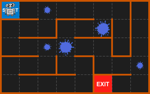
Baby Robot now has a challenging problem, where he must search the maze looking for the exit. When the standard Gym Environment Reinforcement Learning loop is run, Baby Robot will begin to randomly explore the maze, gathering information that he can use to learn how to escape. Part of one of these episodes is shown in Figure 15 below.

Obviously, given that random actions are being taken, and with the added complication of puddles that can potentially cause skids, it may take Baby Robot some time to locate the exit. To see how a Reinforcement Learning algorithm can be used to find the best route through the maze, check out the training notebook.

Summary

Over the course of these two articles we’ve seen how a custom Gym Environment can be created, with real-time graphical output rendered directly into Jupyter Notebook cells.

The ipycanvas library provides direct access to the HTML canvas, where simple graphical components can be combined to produce informative views of the Reinforcement Learning environment.

Additionally, by basing this environment on the Gym API we can create Reinforcement Learning problems that are compatible with a host of different out-of-the box learning algorithms. Hopefully these articles have given you all the information you need to start building your own, bespoke, RL environments.

If you’d just like to have a play with the Baby Robot environment, check out this notebook showing the different ways in which Baby Robot Grid Worlds can be created and the components that can be added.

Now that we can create a range of challenging worlds for Baby Robot to explore, all that’s left to do is learn how to tackle these problems. The first part of the series on how to do this can be found here: