Create Extraordinary Visualizations with ggplot2 in R

A demonstration using the IBM Telco Churn dataset

ggplot2 demo using a Kaggle dataset. Chart by author

A Call for Better Visualization

Exploratory Data Analysis (“EDA”) has typically been one of the first steps in a data science pipeline. By employing visualization methods and tools, it helps data scientists unpack the relationship between the target variable and various features in the dataset. In addition, when communicating with respect to a technical topic, my experience has been that good visualizations help greatly with story-telling, ultimately adding credibility to my personal brand and building trust with senior stakeholders in the company.

R’s ggplot2

The ggplot2 package is a dedicated package in R for data visualizations. The “gg” in ggplot2 stands for Grammar of Graphics. Apart from the bivariate EDA which shows a ‘one-way’ relationship between the target variable and a single feature, the ggplot2 package allows for multivariate EDA with its faceting customizations, which I’ll demonstrate in later sections of this article. More importantly, and as you can see in this link which showcases the possibilities, ggplot2 is best known for its stunning visuals. The charts below provide some examples of what ggplot2 is capable of.

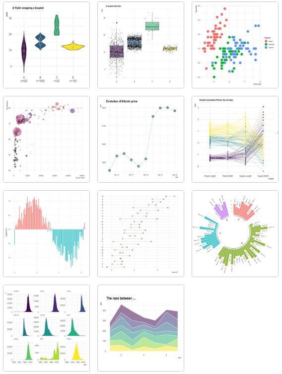
Image 1: ggplot2 possibilities. Source: R Graph Gallery

With the bivariate or multivariate relationship visualized before the fitting of a predictive model, users are able to justify in the first instance the inclusion of certain features (or even exclusion of certain features which show no clear relationship with the target variable).

The Dataset

The dataset I’ll be using to support the case for using the ggplot2 package is the commonly known IBM Telco Churn dataset. It contains 20 independent features and 1 target variable “Churn” which indicates whether the customer discontinued using the Telco’s service. It was initially purposed to train a classification model which predicts the target variable.

This dataset was sourced from Kaggle and represents an adaptation of the original IBM dataset. A data dictionary for this dataset is provided in the table below. All features are categorical apart from tenure, MonthlyCharges (i.e. monthly premiums) and TotalCharges.

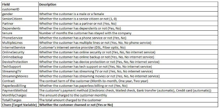
Table 2: Data dictionary. Table by author

For the purpose of this article, I’ll be demonstrating the plotting of chart types such as histograms, density plots, box plots and Stat2D plots with ggplot2 using a subset of numerical as well as categorical features in the dataset.

Distribution of Target Variable by Features

The main purpose of performing an EDA is to understand whether a particular feature is useful in predicting the target variable. This can be achieved by examining the distribution of the target variable by this feature. For instance, the hypothesis may be that the distribution of churn is skewed towards customers who paid higher MonthlyCharges, or customers who paid the Telco using the Electronic Cheque PaymentMethod. Let’s see if we can validate these hypotheses with the ggplot2 visualizations.

ETL

For readers not familiar with R, some ETL needs to happen before we start plotting. The steps are:

## Import Libraries
library(ggplot2)
library(dplyr) # for filtering

## Load data
data_raw <- read.csv('Path/WA_Fn-UseC_-Telco-Customer-Churn.csv', header = TRUE)

## Apply filters - "if" stands for inforce
data_if    <- data_raw %>% 
  filter(`Churn` == "No")
data_churn <- data_raw %>%
  filter(`Churn` == "Yes")

Effectively with these steps we ingested and split the dataset by churned and inforce customers (i.e. customers who departed vs. customers who stayed).

Demonstration 1 — Distribution of Churn by MonthlyCharges

Chart 3: Distribution of Churn by MonthlyCharges. Chart by author

The R code for creating Chart 3 is provided below. In particular:

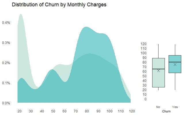
A density plot is shown on the left hand side of the frame, and a box plot is shown on the right hand side of the frame. The two plots occupy circa. 74% and 26% of the frame respectively as customized by the ggarrange function under the ggpubr library.
In the density plot, the teal (i.e. lighter) color represents the distribution of MonthlyCharges for the inforce customers, compared against the aqua (i.e. darker) color which represents the distribution of MonthlyCharges for the churned customers. They are plotted on the same scale and therefore are easily comparable. The level of transparency for the overlapped areas is customized to 0.6 (or 60%) by the alpha argument in the geom_density code.
In the box plot, the 25ᵗʰ, 50ᵗʰ and 75ᵗʰ percentiles, as well as the mean (denoted by the cross) of MonthlyCharges for the inforce and churned customers are shown and can be easily compared.
Customizations of the chart can be extended to the setting of labels (including units and breaks) for the x and y axis, titles for the chart, legend and axis, background colors, font type and size, and more. A complete list of customizations of the ggplot2 aesthetics can be explored here.

From this chart, the key observations are:

Based on the density plot, MonthlyCharges paid by customers ranged from $20 — $120 in the dataset.
Based on the box plot, customers who departed paid circa. $20 higher MonthlyCharges compared to customers who stayed.
The distribution of churned customers was skewed towards higher MonthlyCharges, particularly customers who paid MonthlyCharges > $70, whereas the distribution of inforce customers was skewed towards lower MonthlyCharges, particularly customers who paid MonthlyCharges <$30.

These observations collectively depict a story that customers who departed were generally on more expensive ‘plans’ with the Telco.

## Import Library for plot aggregation
library(ggpubr)

limit_prem <- 120
den_prem <- ggplot() + 
  geom_density(data = data_if, aes(x = data_if[["MonthlyCharges"]], y = ..count../sum(..count..)), fill = "#AAD8C8", alpha = 0.6, color = NA) +
  geom_density(data = data_churn, aes(x = data_churn[["MonthlyCharges"]], y = ..count../sum(..count..)), fill = "#2FB3B6", alpha = 0.6, color = NA) +
  
scale_x_continuous(labels = comma, breaks = seq(0, limit_prem, 10) 
  #                   , guide = guide_axis(n.dodge = 2)
                   ) +
scale_y_continuous(labels = percent, breaks=seq(0, 0.006, 0.001)) +
  theme(
        axis.title = element_blank(),
        legend.position = "bottom",
        legend.title = element_blank(),
        legend.text = element_text(size = 8)
        ) +
  labs(
       title = "Distribution of Churn by Monthly Charges") +
  theme(panel.background = element_rect(fill = '#FFFFFF', color = "#FFFFFF"),
        panel.grid.major.x = element_blank(),
        panel.grid.minor = element_blank(),
        axis.ticks = element_blank() )

box_prem <- ggplot(data_raw, aes(x = as.factor(data_raw[["Churn"]]), y = data_raw[["MonthlyCharges"]], fill = as.factor(data_raw[["Churn"]]))) + 
  geom_boxplot(outlier.colour=NA, alpha = 0.6) +
  scale_y_continuous(labels = comma, breaks=seq(0, limit_prem, 10)
                     #, guide = guide_axis(n.dodge = 2)
                     ) +
  coord_cartesian(ylim = c(0, 200)) +
  theme(legend.title = element_blank(),
        legend.position = "none"
        ) +
  labs(x = "Churn") +
  theme(panel.background = element_rect(fill = '#FFFFFF', color = "#FFFFFF"),
        panel.grid.major.x = element_blank(),
        panel.grid.major.y = element_blank(),
        panel.grid.minor = element_blank(),
        axis.ticks = element_blank(),
        axis.title.y = element_blank(),
        axis.title.x = element_text(size = 8),
        axis.text.x = element_text(size = 8)
        ) +
  scale_fill_manual(values=c("#AAD8C8", "#2FB3B6")) +
  stat_summary(fun = "mean", shape = 4, color = "#303E46")

# Embedding the density and box plots into one frame
ggr_prem_den <- ggarrange(den_prem, box_prem, widths = c(2.0, 0.7),
          ncol = 2, nrow = 1)

print(ggr_prem_den)

Demonstration 2 — Distribution of Churn by Tenure (Months)

For another numerical feature tenure, similar charts can be created by replacing the feature name “MonthlyCharges” in the R code above with “tenure” (and modifying the units on the x-axis).

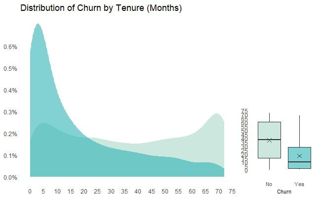
Chart 4: Distribution of Churn by Tenure. Chart by author

From this chart, the key observations are:

There was evidence that the distribution of churn was skewed towards customers with lower tenures. That is, churn was more likely to occur to customers who stayed with the Telco for a relatively short period of time, possibly supporting a case for retention campaign by the Telco which focuses on this customer segment.
There were proportionally less churns for customers who had stayed with the Telco for more than 24 months.
Given the relatively clean-cut relationship, it’s likely that tenure will be an important feature in predicting customer churn, and therefore should be included for (at least the initial) model fitting post EDA.

Demonstration 3 — Distribution of Churn for Categorical Variables

The chart below shows the distribution of churn by a number of categorical features in the dataset. Similar to the density plots for the numerical variables shown previously, the two distributions (for the inforce and churned customers) are plotted on the same scale so that they can be easily compared.

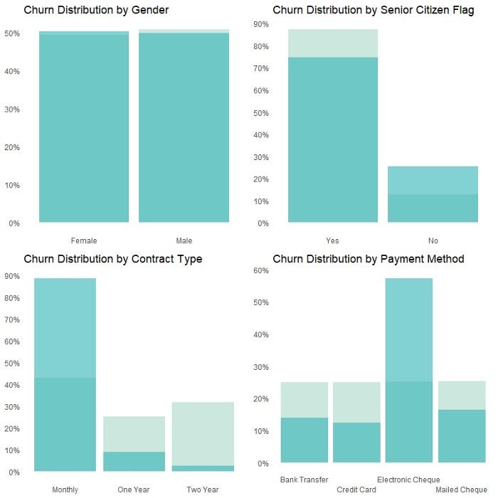
Chart 5: Distribution of Churn by Gender, Senior Citizen Flag, Contract Type and Payment Method. Chart by author

Histograms are used to create the chart above as they are more suitable for categorical features compared to density plots (which are more suitable for numerical features). The R code for creating the chart for the categorical feature PaymentMethod is provided below. Charts for other categorical features in the dataset can be easily replicated by modifying the call to the feature name and the x-axis label in the code.

labels_PM <- c("Bank Transfer", "Credit Card", "Electronic Cheque", "Mailed Cheque")

PM_hist <- ggplot() + 
  geom_bar(data = data_if, aes(x = as.factor(data_if[["PaymentMethod"]]), y = ..count../sum(..count..)), fill = "#AAD8C8", alpha = 0.6) +
    geom_bar(data = data_churn, aes(x = as.factor(data_churn[["PaymentMethod"]]), y = ..count../sum(..count..)), fill = "#2FB3B6", alpha = 0.6) +
  scale_y_continuous(labels = scales::percent, breaks = seq(0, 1, 0.1)) +
  scale_x_discrete(labels = labels_PM, guide = guide_axis(n.dodge = 2)) +
  theme(axis.title = element_blank()) +
  theme(legend.title = element_blank(),
        legend.position = "none") +
  labs(title = "Churn Distribution by Payment Method") +
  theme(panel.background = element_rect(fill = '#FFFFFF', color = "#FFFFFF"),
        panel.grid.major.x = element_blank(),
        panel.grid.major.y = element_blank(),
        panel.grid.minor = element_blank(),
        axis.ticks = element_blank(),
        axis.title.y = element_blank(),
        axis.title.x = element_blank(),
        axis.text.x = element_text(size = 9))

print(PM_hist)

From this chart, the key observations are:

There were proportionally higher churns for customers who were a Senior Citizen, on a Monthly Contract or had a payment method of Electronic Cheque.
Distribution of churn did not seem to differentiate by Gender.

It may be worth digging into customer segments with materially higher proportion of churns, for example, customers who paid by Electronic Cheque.

Overlaying the histogram for PaymentMethod with a Stat2D plot which shows another dimension of customers by MonthlyCharges and PaymentMethod suggests that customers who paid by Electronic Cheque were associated with higher MonthlyCharges, as denoted by the darker region in the $80 — $110 range in the Stat2D plot. This supports a story that higher churns for payments by Electronic Cheque could be related to higher MonthlyCharges these customers were paying.

The extent of this can then be unpacked at the modelling stage. Nonetheless, the charts effectively display a three-way relationship between the target variable and PaymentMethod as well as MonthlyCharges.

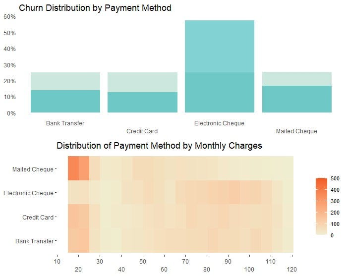
Chart 6: Distribution of Churn by Payment Method (top), overlayed with Stat2D plot for MonthlyCharges by Payment Method (bottom). Chart by author

The R code for creating the above Stat2D plot is provided below.

labels_y_payment_method <- c("Bank Transfer", 
                           "Credit Card", 
                           "Electronic Cheque",
                           "Mailed Cheque")

Stat2D_tenure_PM <- ggplot(data_if, aes(x = `tenure`, y = `PaymentMethod`)) +
  stat_bin2d(bins = 20) +
  scale_fill_gradient(low = "#EFEFD2", high = "#F15A24", limits = c(0, 500)) +
 scale_x_continuous(labels = comma, breaks=seq(0, 120, 10)
                     ,guide = guide_axis(n.dodge = 2)
                     ) +
 scale_y_discrete(labels = labels_y_payment_method) +
  theme(axis.title = element_blank(),
        legend.position = "right",
        legend.title = element_blank(),
        legend.text = element_text(size = 8)
        ) +
  labs(title = "Distribution of Payment Method by Tenure (Months)") +
  theme(panel.background = element_rect(fill = '#FFFFFF', color = "#FFFFFF"),
        panel.grid.major.x = element_blank(),
        panel.grid.major.y = element_blank(),
        panel.grid.minor = element_blank(),
        ) 
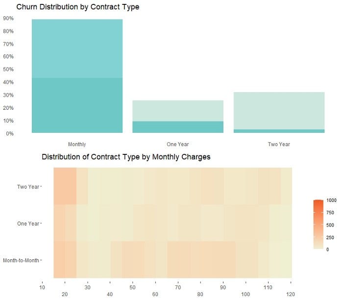
print(Stat2D_tenure_PM)

Similar charts can be created for customers who were on a Monthly Contract Term, as shown below. To a lesser extent, customers who were on a Monthly Contract were were also associated with higher MonthlyCharges.

Chart 7: Distribution of Churn by Contract Type (top), overlayed with a Stat2D plot for MonthlyCharges by Contract Type (bottom). Chart by author

Demonstration 4 — Faceting

Another way to visualize a three-way relationship with ggplot 2 is through faceting. The facet chart below shows MonthlyCharges by ContractType and PaymentMethod.

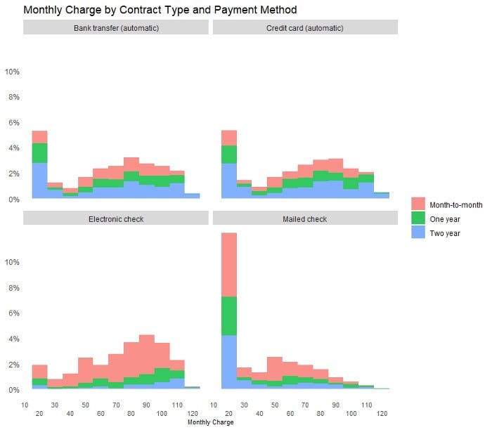
Chart 7: Facet Chart Monthly Charge by Contract Type and Payment Method. Chart by author

It can be observed that:

Number of customers were evenly distributed by the four payment methods.
Customers who paid by Electronic Cheque had proportionally higher Monthly Charge compared to customers who paid by other Payment Methods.
Much higher portion of customers who paid by Electronic Cheque held a Monthly Contract compared to customers who paid by other Payment Methods.
Distribution of attributes was surprisingly similar between customers who paid by Bank Transfer and Credit Card.
There may be an outlier in the dataset for customers who paid by Mailed Cheque, and who paid Monthly Charges in the $20 — $25 range, as indicated by the bar of abnormal height in the chart.

The R code for creating the facet chart is provided below.

facet_monthly_charge <- ggplot() + 
  geom_histogram(data = data_if, aes(x = data_if[["MonthlyCharges"]], y = ..count../sum(..count..), fill = data_if[["Contract"]]), alpha = 0.8, color = NA, binwidth = 10) +
  facet_wrap("PaymentMethod") +
  scale_x_continuous(labels = comma, breaks = seq(0, limit_prem, 10), 
                   guide = guide_axis(n.dodge = 2)
                   ) +
  scale_y_continuous(labels = percent, breaks=seq(0, 0.1, 0.02)) +
  theme(legend.title = element_blank(),
        legend.position = "right"
        ) +
  labs(x = "Monthly Charge",
       title = "Monthly Charge by Contract Type and Payment Method") +
  theme(
        panel.background = element_rect(fill = '#FFFFFF', color = "#FFFFFF"),
        panel.grid.major.x = element_blank(),
        panel.grid.major.y = element_blank(),
        panel.grid.minor = element_blank(),
        axis.ticks = element_blank(),
        axis.title.y = element_blank(),
        axis.title.x = element_text(size = 8),
        axis.text.x = element_text(size = 8))

print(facet_monthly_charge)

Concluding Thoughts

I am a strong believer that visualization is an extremely important tool in telling a convincing story to senior stakeholders and decision makers. There is a reason why the Big 4 consultants get paid a premium to do what they do, and this to me is partly because they have better visualization templates when it comes to presenting and communicating to their clients.

With great packages like ggplot2, this article hopefully provides a guide for those who, like myself, are particular about and want to achieve great things with visualizations.

I have previously blogged about other visualization techniques in the following articles. If you like these, make sure you follow the writer on Medium!

Interactive Geospatial Visualization with Shape Map Visual in PowerBI

Creating Interactive Geospatial Visualisation with Python

As I ride the AI/ML wave, I enjoy writing and sharing step-by-step guides and how-to tutorials in a comprehensive language with ready-to-run codes. If you would like to access all my articles (and articles from other practitioners/writers on Medium), you can sign up using the link here!