Correlation between Market Index and Stocks

Photo by Pietro Jeng on Unsplash.com

The other day I wrote a post about analyzing the correlation between two crypto coin prices to see if their price movement is related. In this article I would like to take a slightly different direction and discuss the correlation between a market index and different stocks.

Every trader has experienced the effect of the value of his positions plummeting when there is a sudden market downturn. If we could quantify the correlation between the market and our holdings, it would allow us to diversify our portfolio by picking stocks that have a positive and negative relationship to the market.

Taking things a step further, if we find assets that very closely follow the market trends, we may be able to get signals of trend reversals from the market index and make buy/sell decisions based on those signals.

This story is solely for general information purposes, and should not be relied upon for trading recommendations or financial advice. Source code and information is provided for educational purposes only, and should not be relied upon to make an investment decision. Please review my full cautionary guidance before continuing.

What is Correlation?

Correlation is statistical relation ship of dependence between two variables or data sets. In statistics, correlation often refers to the degree in which two variables are linearly related.

In this post we are going to examine the correlation of prices, in particular the relation between the prices of a market index and different stocks.

Trade Ideas provides AI stock suggestions, AI alerts, scanning, automated trading, real-time stock market data, charting, educational resources, and more. Get a 15% discount with promo code ‘BOTRADING15’.

Visual Correlation

The easiest way to check the correlation of an investment asset to a market index is by plotting them out in a chart. By plotting them together, we can immediately tell if their price movement are closely related, somewhat or not at all.

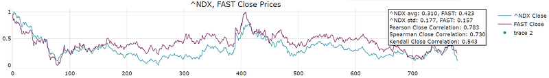
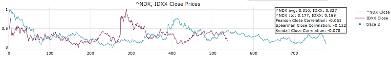
In the graph below we plotted 1-minute prices of two stocks, INDEXX Laboratories, Inc (IDXX) and Fastenal Corporation (FAST) against the NASDAQ Composite Index. The two stocks are both part of that index.

The price data has been normalized to remove the difference in scale between the prices to be compared.

Here you see that the Close price of Fastenal seems to match the Close price of the NASDAQ 100 index very closely.

In contrast, the Close price of INDEXX Laboratories doesn’t seem to match NASDAQ 100 at all.

Scatterplots

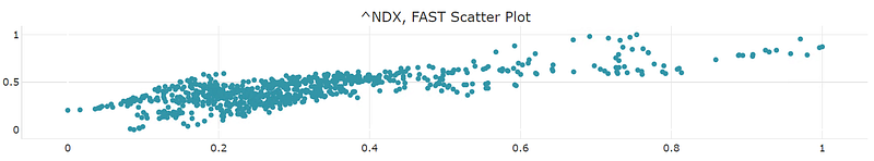
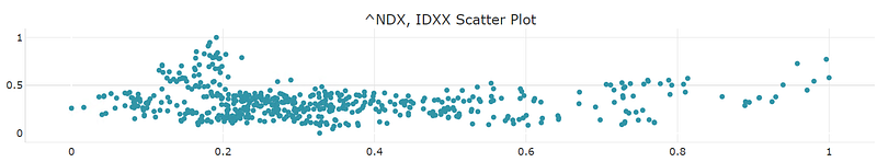
Another way to analyze linear correlation between two values is to plot them out in a scatter plot.

When plotting the close prices of Fastenal and the NADAQ 100, we see a clear linear relationship and can imagine a that the dots align with a diagonal line drawn through the center of the dot distribution.

When plotting the close prices of INDEXX and the NASDAQ 100, it seems that the dots are randomly scattered around the graph.

Pearson Correlation

So far we have used visualization to assess a relationship between variables but what if we actually want to quantity the relationship in a precise value?

The Pearson correlation — invented by Karl Pearson — is used to assess the quality of a linear relationship between two sets of data. It is calculated as the covariance of the two variables divided by the product of the standard deviation of each data set.

Pearson’s correlation = covariance(X, Y) / (std(X) * std(Y))

The coefficient that is calculated by this formula returns values between -1 and 1. A value of -1 represents a complete negative correlation, whereas a value of 0 represents no correlation at all and 1 represents full positive correlation.

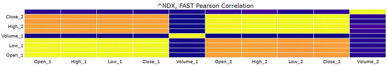
The Pearson value I calculated for Fastenal is 0.783, so a very close positive correlation. This is also apparent in the heatmap below. The map has a light orange color where Close_1 (Fastenal Close) and Close_2 (NADAQ 100) intersect, which indicates a close positive relation.

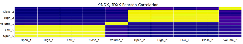
The Pearson coefficient for INDEXX is -0.63 so a slightly negative correlation. This is also indicated in the heatmap by the dark purple color, where Close_1/Close_2 intersect.

Spearman Correlation

The Spearman Correlation is another measure of the relationship between two variables or data sets invented by Charles Spearman. It assesses how well the relationship between two variables can be described using a monotonic function. A monotonic function is a function between dataset that preserves or reverses the given order.

As with the Pearson correlation coefficient, the scores range between -1 and 1. The meaning of the range is the same as for the Pearson Correlation.

The Spearman Correlation Coefficient is calculated from the relative rank of values on each sample. This is a common approach used in non-parametric statistics, e.g. statistical methods where we do not assume a distribution of the data such as Gaussian.

Spearman’s correlation coefficient = covariance(rank(X), rank(Y)) / (std(rank(X)) * std(rank(Y)))

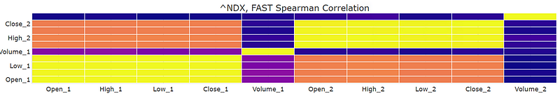
For the Spearman coefficient I calculated for Fastenal was 0.73 so again a high positive correlation.

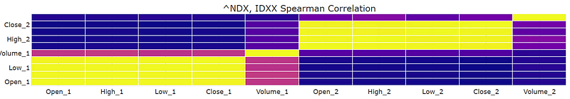
For the Spearman coefficient for INDEXX was -0.122, which represents a slightly negative correlation.

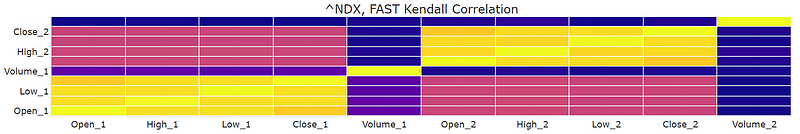
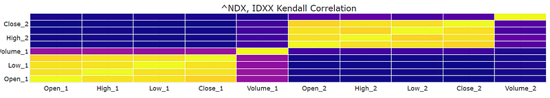
Kendall Correlation

A third method for assessing the relationship between variables is the Kendall Correlation rank coefficient, named after Maurice Kendall. It is used to measure the ordinal association between two measured quantities.

Here the formula for the Kendall coefficient:

Source: Wikipedia, Creative Commons License 3.0

The Kendall coefficient for Fastenal is 0.54, which represents a positive correlation.

The Kendall coefficient for INDEXX is -0.078, which represents a slightly negative correlation.

Python Implementation

The analysis above can be implemented using the following Python libraries:

• pandas
• numpy
• sklearn
• yfinance
• pandas_ta.

If you would like to learn how to code this analysis in Python, look out for my next post.

Wrapping Up

In this post we looked at the different ways to assess correlation between a market index and different stocks.

I hope you found this post worth your time. Thanks for reading.

You can support my writing for free using this link. Don’t miss another story — subscribe to my stories by email. For more premium content, check out my ‘B/O Trading Blog’ on Substack.

This post contains affiliate marketing links.

Have a great day!