Cooking your first U-Net for Image Segmentation

Fellow AI cooks, today you are going to learn how to prepare one of the most important recipes in Computer Vision: the U-Net.

You can find the full code on my Github, or on Google Colab

Even better, we are going to apply the U-Net to the MRI segmentation dataset from Kaggle, accessible here:

Brain MRI segmentation

Brain MRI images together with manual FLAIR abnormality segmentation masks

www.kaggle.com

Ingredients of the Recipe:

Exploration of the Dataset
Creation of the Datasets and Dataloader classes
Creation of the architecture
Examining the losses (DICE and Binary Cross Entropy)
Results
Post-cooking tips to Spice things up!

Exploration of the Dataset

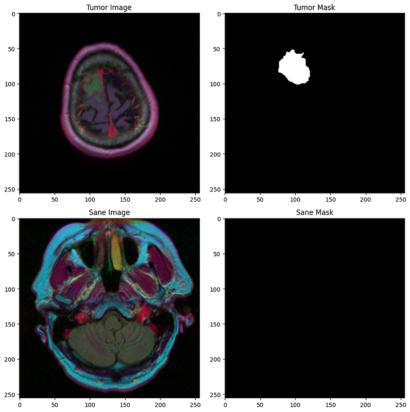
We are given a set of (255 x 255) 2D images of MRI scans, as well as their corresponding masks, where we have to classify each pixel as either 0 (sane), or 1 (tumour).

Here are some examples:

First row: tumour, second row: sane subject

Dataset and DataLoader classes

This is a step that you will find in every project involving a neural network. We

Dataset class

import torch
import torch.nn as nn
import torch.nn.functional as F
from torch.utils.data import Dataset, DataLoader

class BrainMriDataset(Dataset):
    def __init__(self, df, transforms):
        # df contains the paths to all files
        self.df = df
        # transforms is the set of data augmentation operations we use
        self.transforms = transforms
        
    def __len__(self):
        return len(self.df)
    
    def __getitem__(self, idx):
        image = cv2.imread(self.df.iloc[idx, 1])
        mask = cv2.imread(self.df.iloc[idx, 2], 0)
        
        augmented = self.transforms(image=image, 
                                    mask=mask)
 
        image = augmented['image'] # Dimension (3, 255, 255)
        mask = augmented['mask']   # Dimension (255, 255)

        # We notice that the image has one more dimension (3 color channels), so we have to one one "artificial" dimension to the mask to match it
        mask = np.expand_dims(mask, axis=0) # Dimension (1, 255, 255)
        
        return image, mask

Dataloader

Now that we have create the Dataset class to reshape the tensors, we need to first define the train set (used to train the model), the validation set (used to monitor training and avoid overfitting), and a test set to finally evaluate the performance of our model on unseen data.

# Split df into train_df and val_df
train_df, val_df = train_test_split(df, stratify=df.diagnosis, test_size=0.1)
train_df = train_df.reset_index(drop=True)
val_df = val_df.reset_index(drop=True)

# Split train_df into train_df and test_df
train_df, test_df = train_test_split(train_df, stratify=train_df.diagnosis, test_size=0.15)
train_df = train_df.reset_index(drop=True)

train_dataset = BrainMriDataset(train_df, transforms=transforms)
train_dataloader = DataLoader(train_dataset, batch_size=32, shuffle=True)

val_dataset = BrainMriDataset(val_df, transforms=transforms)
val_dataloader = DataLoader(val_dataset, batch_size=32, shuffle=False)

test_dataset = BrainMriDataset(test_df, transforms=transforms)
test_dataloader = DataLoader(test_dataset, batch_size=32, shuffle=False)

The U-Net Architecture

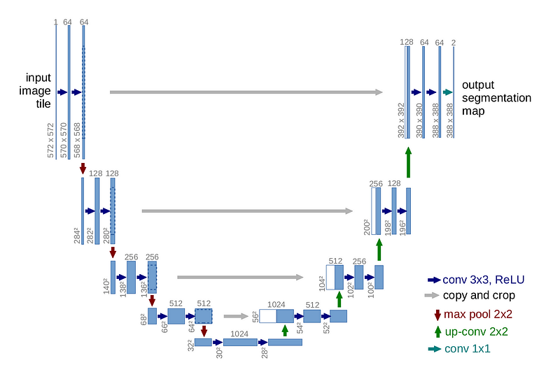
The U-Net architecture, a powerful model for image segmentation tasks, is a type of Convolutional Neural Network (CNN) that gets its name from its U-shaped structure. The U-Net was first developed by Olaf Ronneberger et al. in their 2015 paper titled “U-Net: Convolutional Networks for Biomedical Image Segmentation.”

Its structure involves an encoding (downsampling) path and a decoding (upsampling) path.

The U-Net is still a very successful model nowadays, and its success comes from 2 main ingredients:

Its symmetric structure (U Shape)
The forward connections (gray arrows on the picture)

The main idea of the forward connection is that as we go deeper and deeper in the layers, we lose some information about the original image. However our task is to segment the image, and we need precisely the image to classify every pixel. This is why we reinject the image at each layer of the encoding layer in the symmetric decoder layer.

Here is how to code it in Pytorch:

train_dataset = BrainMriDataset(train_df, transforms=transforms)
train_dataloader = DataLoader(train_dataset, batch_size=32, shuffle=True)

val_dataset = BrainMriDataset(val_df, transforms=transforms)
val_dataloader = DataLoader(val_dataset, batch_size=32, shuffle=False)

test_dataset = BrainMriDataset(test_df, transforms=transforms)
test_dataloader = DataLoader(test_dataset, batch_size=32, shuffle=False)


class UNet(nn.Module):

    def __init__(self):
        super().__init__()

        # Define convolutional layers
        # These are used in the "down" path of the U-Net,
        # where the image is successively downsampled
        self.conv_down1 = double_conv(3, 64)
        self.conv_down2 = double_conv(64, 128)
        self.conv_down3 = double_conv(128, 256)
        self.conv_down4 = double_conv(256, 512)

        # Define max pooling layer for downsampling
        self.maxpool = nn.MaxPool2d(2)

        # Define upsampling layer
        self.upsample = nn.Upsample(scale_factor=2, mode='bilinear', align_corners=True)

        # Define convolutional layers
        # These are used in the "up" path of the U-Net,
        # where the image is successively upsampled
        self.conv_up3 = double_conv(256 + 512, 256)
        self.conv_up2 = double_conv(128 + 256, 128)
        self.conv_up1 = double_conv(128 + 64, 64)

        # Define final convolution to output correct number of classes
        # 1 because there are only two classes (tumor or not tumor)
        self.last_conv = nn.Conv2d(64, 1, kernel_size=1)

    def forward(self, x):
        # Forward pass through the network

        # Down path
        conv1 = self.conv_down1(x)
        x = self.maxpool(conv1)
        conv2 = self.conv_down2(x)
        x = self.maxpool(conv2)
        conv3 = self.conv_down3(x)
        x = self.maxpool(conv3)
        x = self.conv_down4(x)

        # Up path
        x = self.upsample(x)
        x = torch.cat([x, conv3], dim=1)
        x = self.conv_up3(x)
        x = self.upsample(x)
        x = torch.cat([x, conv2], dim=1)
        x = self.conv_up2(x)
        x = self.upsample(x)
        x = torch.cat([x, conv1], dim=1)
        x = self.conv_up1(x)

        # Final output
        out = self.last_conv(x)
        out = torch.sigmoid(out)

        return out

Losses and Evaluation Criterion

Like every neural network, there is an objective function, a loss, that we minimize with gradient descent. We also introduce the evaluation criterion, that help us to train the model (if it does not improve over let’s say 3 consecutive epochs, then we strop training becaue th emodel is overfitting).

Here there are two main things to retain from this paragraph:

The loss function is a combination of two losses function (DICE loss, Binary Cross-Entropy)
The Evaluation function is the DICE score, not to be mixed up with the DICE loss

If you made it so far, congratulations! You have done the hardest. Now let’s train the model and observe the results.

DICE Loss:

Remark: we add a smoothing parameter (epsilon) to avoid the division by zero.

Binary Cross Entropy Loss:

Finally our total loss is:

Let’s implement it together:

def dice_coef_loss(inputs, target):
    smooth = 1.0
    intersection = 2.0 * ((target * inputs).sum()) + smooth
    union = target.sum() + inputs.sum() + smooth

    return 1 - (intersection / union)


def bce_dice_loss(inputs, target):
    inputs = inputs.float()
    target = target.float()
    
    dicescore = dice_coef_loss(inputs, target)
    bcescore = nn.BCELoss()
    bceloss = bcescore(inputs, target)

    return bceloss + dicescore

Evaluation criterion (Dice Coefficient):

The Evaluation function we use is the DICE score. It is between 0 and 1, and 1 is the best.

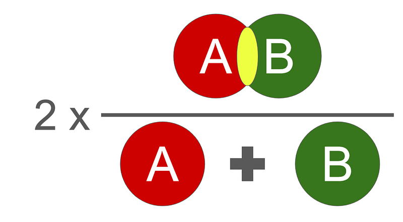
Its mathematical implementation is the following:

def dice_coef_metric(inputs, target):
    intersection = 2.0 * (target * inputs).sum()
    union = target.sum() + inputs.sum()
    if target.sum() == 0 and inputs.sum() == 0:
        return 1.0

    return intersection / union

Training Loop

def train_model(model_name, model, train_loader, val_loader, train_loss, optimizer, lr_scheduler, num_epochs):  
    
    print(model_name)
    loss_history = []
    train_history = []
    val_history = []

    for epoch in range(num_epochs):
        model.train()  # Enter train mode
        
        # We store the training loss and dice scores
        losses = []
        train_iou = []
                
        if lr_scheduler:
            warmup_factor = 1.0 / 100
            warmup_iters = min(100, len(train_loader) - 1)
            lr_scheduler = warmup_lr_scheduler(optimizer, warmup_iters, warmup_factor)
        
        # Add tqdm to the loop (to visualize progress)
        for i_step, (data, target) in enumerate(tqdm(train_loader, desc=f"Training epoch {epoch+1}/{num_epochs}")):
            data = data.to(device)
            target = target.to(device)
                      
            outputs = model(data)
            
            out_cut = np.copy(outputs.data.cpu().numpy())

            # If the score is less than a threshold (0.5), the prediction is 0, otherwise its 1
            out_cut[np.nonzero(out_cut < 0.5)] = 0.0
            out_cut[np.nonzero(out_cut >= 0.5)] = 1.0
            
            train_dice = dice_coef_metric(out_cut, target.data.cpu().numpy())
            
            loss = train_loss(outputs, target)
            
            losses.append(loss.item())
            train_iou.append(train_dice)

            # Reset the gradients
            optimizer.zero_grad()
            # Perform backpropagation to compute gradients
            loss.backward()
            # Update the parameters with the computed gradients
            optimizer.step()
    
            if lr_scheduler:
                lr_scheduler.step()
        
        val_mean_iou = compute_iou(model, val_loader)
        
        loss_history.append(np.array(losses).mean())
        train_history.append(np.array(train_iou).mean())
        val_history.append(val_mean_iou)
        
        print("Epoch [%d]" % (epoch))
        print("Mean loss on train:", np.array(losses).mean(), 
              "\nMean DICE on train:", np.array(train_iou).mean(), 
              "\nMean DICE on validation:", val_mean_iou)
        
    return loss_history, train_history, val_history

Results

Let’s evaluate our model on a subject with a tumour:

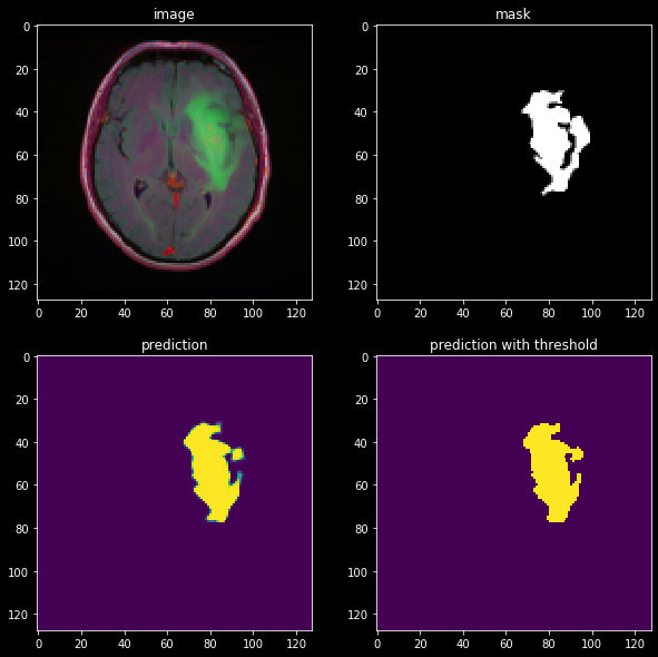
The result looks pretty good! We can see that the model has definetly learned some useful information about the structure of the image. However it could refine the segmentation better, and that can be achieved with more advanced techniques that we will review soon.

The U-Net is still widely used today, but there is one famous model that reaches state of the art performance called the nn-UNet. You should definetly check The Ultimate Guide to nnU-Net

Thanks for reading! Before you go:

Check my compilation of AI tutorials on Github

GitHub — FrancoisPorcher/awesome-ai-tutorials: The best collection of AI tutorials to make you a…

The best collection of AI tutorials to make you a boss of Data Science! — GitHub …

github.com

You should get my articles in your inbox. Subscribe here.

If you want to have access to premium articles on Medium, you only need a membership for $5 a month. If you sign up with my link, you support me with a part of your fee without additional costs.

If you found this article insightful and beneficial, please consider following me and leaving a clap for more in-depth content! Your support helps me continue producing content that aids our collective understanding.

Post-cooking Tips to Spice things up!

If you have made it until now, congratulations! If you want to spice-up the final meal, here are some interesting ressources to look at:

Semantic vs Instance segmentation
There are other losses used in image segmentation, for example Jaccard loss, Focal loss
If 2D Image Segmentation was too easy for you, you can look at the 3D image segmentation which is much harder because the models are much bigger.
nnUNet, the state-of-the art in a lot of different domains. This neural network does not introduce groundbreaking new features since the U-Net, however it is extremely well engineered, and test different configurations of UNet, and ensembles them to build the strongest baseline possible.

References

Ronneberger O., Fischer P., Brox T. (2015) U-Net: Convolutional Networks for Biomedical Image Segmentation. In: Navab N., Hornegger J., Wells W., Frangi A. (eds) Medical Image Computing and Computer-Assisted Intervention — MICCAI 2015. MICCAI 2015. Lecture Notes in Computer Science, vol 9351. Springer, Cham. https://doi.org/10.1007/978-3-319-24574-4_28
https://www.kaggle.com/datasets/mateuszbuda/lgg-mri-segmentation
https://www.kaggle.com/code/bonhart/brain-mri-data-visualization-unet-fpn
Isensee, Fabian, Paul F. Jaeger, Simon AA Kohl, Jens Petersen, and Klaus H. Maier-Hein. “nnU-Net: a self-configuring method for deep learning-based biomedical image segmentation.” Nature methods 18, no. 2 (2021): 203–211.