Convolutional Neural Networks (CNN) in Keras (TensorFlow) Step by Step Guide

A practical tutorial on image classification with CNN. Code included.

Intro

As promised, this is a follow-up about a convolutional neural network (CNN) using Keras.

As usual, I will describe an important technical background and show how to practically implement this knowledge in the code.

In the previous article, we have already seen the power of a neural network (NN) in classifying images by their labels. If you have missed that article, no worries, I will quickly recap the main ideas.

In case, you are interested in learning more about Keras/TensorFlow and general good principles of building your own NN, I would suggest looking into this article:

When working with images, it is not enough to simply use flattened and dense (fully connected) layers.

To make our analysis as robust as possible, we better make use of any available information about our data. In the case of images, it is the 2D pixel distribution.

In other words, we were classifying images without using any structural information hidden within the images.

So, the main goal of this article is to improve my previous NN by transforming it into a CNN.

To make the whole process easier, let us divide it into steps:

1. Briefly explain how CNN works;
2. Recap a dataset we will be working on;
3. Create our own CNN architecture with Keras;
4. Train and test our model;
5. Compare to the usual NN.

Let us begin.

Step 1. What is CNN and how does it work?

In very simple words,

CNN is a process of transforming original data into a feature map by applying an operation of convolution.

Mathematically speaking, convolution is an operation on two functions that produces a third function. That third function shows how the shape of one is modified by the other.

Intuitively, every subsequent convolution layer in the CNN is a simpler version of the previous layer. In this process, we (ideally) get reduced data without losing any important features present in the original data.

To illustrate this process, I prepared a small animation:

Technically, the convolution performs a pixel-wise multiplication of the filter with the portion of the image and then sums up the result. Then, the filter is moved to the next portion of the image so this operation repeats.

Convolution is an interesting process and it can be explored in more detail, however, the goal of this article is to showcase how to build our own CNN in Keras.

Note: The layers of CNN are not fully connected, such as in more classical dense layers.

Let us now move on to the actual data and CNN architecture and first of all import the initial list of libraries and methods needed for this tutorial.

Step 2. Data Set (recap)

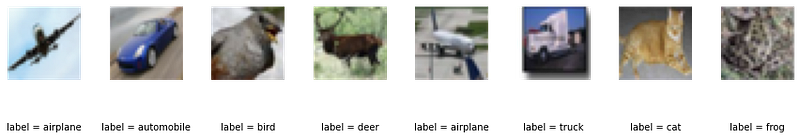
As an example, we will be classifying images using a famous CIFAR-10 dataset, which is already included in the Keras library.

This data set consists of 60k 32 by 32 pixels color images, with 10 classes:

airplane, automobile, bird, cat, deer, dog, frog, horse, ship, truck

For more detail about this data set, please take a look at my previous article.

Here is a short script for visualizing this dataset.

As a result, we can see something like that:

Now, let us move on to the most important section of this project — CNN architecture in Keras.

Step 3. Create our own CNN in Keras

If I were to summarize the Keras CNN architecture, I would mention the following elements

• the number of CNN layers;
• the number of filters/kernels;
• the stride size;
• the padding.

Now, let me briefly describe each of these elements and show the coding part right after that.

The number of CNN layers determines how deep the NN will be.

More layers = deeper but slower NN.

So, better to always start with a smaller number of layers and increase them as we need. In this way, we will only benefit from the NN/CNN as it will not be as heavy to eat up all of our computational resources and will save us a lot of time.

The number of filters/kernels defines a number of convolutions performed on each layer.

More filters = more channels in the output layer.

Each convolution operation produces a 2D activation map.

The size of strides defines a step size by which to move a filter across the input image.

Larger strides = smaller output layer size.

For example, with the strides = 2 and the input layer of 32 x 32 pixels, the output layer (after convolution) will have 16 x 16 pixels and a larger number of channels.

Padding allows the kernel to extend over the edge of the image by adding zeros as additional edge.

When strides = 1 and padding = 'same' the layer dimensions are unchanged.

It is useful to use padding='same' as it makes it easier to keep track of the dimensions.

Note: It is essential to keep track of the dimensions of the data as it passes through the CNN. To ensure that, I will write a simple formula that defines the dimensions of the data immediately after the convolutional layer: output_dimensions = (batch_size, height, width, filters).

To create a simple CNN with two convolutional layers, we can make a use of sequential NN architecture where we place one layer after another, such as

Let us see what are the dimensions of each layer by calling the model summary() method.

I have got the following output:

Model: "model"
_________________________________________________________________
Layer (type)                 Output Shape              Param #   
=================================================================
input_1 (InputLayer)         [(None, 32, 32, 3)]       0         
_________________________________________________________________
conv2d (Conv2D)              (None, 16, 16, 10)        490       
_________________________________________________________________
conv2d_1 (Conv2D)            (None, 8, 8, 20)          1820      
_________________________________________________________________
conv2d_2 (Conv2D)            (None, 8, 8, 30)          5430      
_________________________________________________________________
flatten (Flatten)            (None, 1920)              0         
_________________________________________________________________
dense (Dense)                (None, 10)                19210     
=================================================================
Total params: 26,950
Trainable params: 26,950
Non-trainable params: 0
_________________________________________________________________

You may try applying the dimensions calculation formula which I defined earlier as a double-check and a mini-exercise. Just, ensure that all the dimensions are what you would like them to be.

The rest of the tutorial is quite straightforward if you followed my previous Keras NN guide.

Let us go through the model training, testing, evaluation and comparison with the classic NN.

Step 4. Train and test our model

To make a comparison fair, I will not change anything in the training and validation process relative to the classic NN.

1. We will compile a model

2. Train the model

Model training looks like that

Epoch 1/10
1563/1563 [==============================] - 15s 9ms/step - loss: 1.9045 - accuracy: 0.3296
Epoch 2/10
1563/1563 [==============================] - 13s 9ms/step - loss: 1.7329 - accuracy: 0.4042
Epoch 3/10
1563/1563 [==============================] - 15s 9ms/step - loss: 1.7177 - accuracy: 0.4153
Epoch 4/10
1563/1563 [==============================] - 22s 14ms/step - loss: 1.7033 - accuracy: 0.4210
Epoch 5/10
1563/1563 [==============================] - 20s 13ms/step - loss: 1.6999 - accuracy: 0.4234
Epoch 6/10
1563/1563 [==============================] - 17s 11ms/step - loss: 1.6886 - accuracy: 0.4254
Epoch 7/10
1563/1563 [==============================] - 16s 10ms/step - loss: 1.6864 - accuracy: 0.4258
Epoch 8/10
1563/1563 [==============================] - 17s 11ms/step - loss: 1.6817 - accuracy: 0.4266
Epoch 9/10
1563/1563 [==============================] - 15s 10ms/step - loss: 1.6763 - accuracy: 0.4343
Epoch 10/10
1563/1563 [==============================] - 16s 10ms/step - loss: 1.6636 - accuracy: 0.4313

3. Evaluate our model

The output is

313/313 [==============================] - 2s 4ms/step - loss: 1.7425 - accuracy: 0.3975

Now, we have reached the point where we can compare the performance of the classic and convolutional NN made in Keras.

Let us see the performance and draw corresponding conclusions.

Step 5. Compare to the usual NN

Based on the evaluation of the classical NN, we got:

accuracy: 0.4964

This time, using CNN, we got only:

accuracy: 0.3975

Surprising result, right?!

Does it mean that the classical NN performs better on image classification than the CNN, which is supposed to learn from the spatial distribution of pixels?

No, it does not. I have two points to tell regarding this result.

1. Firstly, both NNs have a very basic architecture. This may be simply a chance of getting something more accurate with NN than with current CNN.
2. We can still improve our CNN to way outperform our good old NN. While the performance of the NN is probably somewhere near its limit unless we would add many more Dense() layers.

Ruslan, but how can we improve our current CNN?

I will tell you.

If you remember my article about the overfitting of the Deep Neural Networks, the hints might be found there.

Basically, we can include a batch normalization, and dropout layers into our CNN and then talk about performance comparison.

This is supposed to significantly improve our CNN.

Now, let us summarize our findings.

Summary

We conducted an experiment of building two relatively basic Neural Networks, classical NN and convolutional CNN.

Based on the accuracy as the performance evaluation metric, basic NN performed better than the convolutional network with the parameters we have chosen.

This does not mean anything for now, because we can still greatly improve our CNN by adding batch normalization and dropout layers.

If you are interested to know how to practically add these layers, let me know.

Last but not least, if you have any questions or comments, found any error, or would like to connect and simply say “Hi!”, please contact me (below).

I will be happy to hear from you.

I hope you have enjoyed this tutorial and found it helpful.

Are you curious about the emerging field of Prompt Engineering? Grab my new e-book! You will learn and master everything from fundamental concepts to practical tips and real-world applications. Additionally, you will receive a bonus of 300 prompts and some of the free resources to kick-start your AI-driven journey. With all this value packed into one e-book, what is the price? The cost of a cup of coffee! Do not miss out on this opportunity to take your skills to the next level!

Contacts

LinkedIn

I recently started a YouTube channel where I talk about different topics, including data science and AI news, research, and life in general among others. It is a steep learning curve for me but I invite you to check it out here.

Never miss a story, join my mailing list!

GitHub