Convolutional Neural Network (CNN) Architecture Explained in Plain English Using Simple Diagrams

Neural Networks and Deep Learning Course: Part 23

We’ve already discussed one neural network architecture — Multilayer Perceptron (MLP). An MLP is not suitable to use with image data as a large number of parameters are involved in the network even for small images.

Convolutional Neural Networks (CNNs) are specially designed to work with images. They are widely used in the domain of computer vision.

Motivation for CNNs

Here are the two main reasons for using CNNs instead of MLPs when working with image data. These reasons will motivate you to learn more about CNNs.

• To use MLPs with images, we need to flatten the image. If we do so, spatial information (relationships between the nearby pixels) will be lost. So, accuracy will be reduced significantly. CNNs can retain spatial information as they take the images in the original format.
• CNNs can reduce the number of parameters in the network significantly. So, CNNs are parameter efficient.

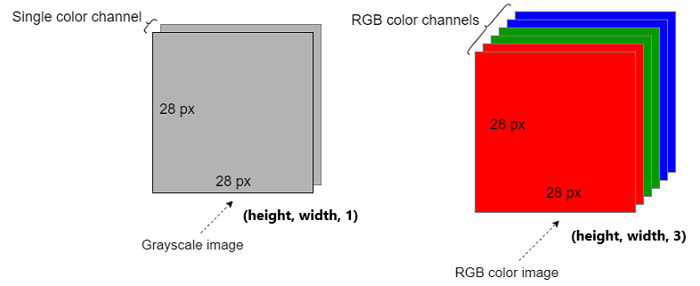
Grayscale vs RGB images (Prerequisite)

CNNs work with both grayscale and RGB images. Before we move on, you need to understand the difference between grayscale and RGB images

An image consists of pixels. In deep learning, images are represented as arrays of pixel values.

There is only one color channel in a grayscale image. So, a grayscale image is represented as (height, width, 1)or simply (height, width). We can ignore the third dimension because it is one. Therefore, a grayscale image is often represented as a 2D array (tensor).

There are three color channels (Red, Green and Blue) in an RGB image. So, an RGB image is represented as (height, width, 3). The third dimension denotes the number of color channels in the image. An RGB image is represented as a 3D array (tensor).

Note: Here are more resources to learn more about grayscale and RGB images.

• How RGB and Grayscale Images Are Represented in NumPy Arrays
• Real-World Examples of 0D, 1D, 2D, 3D, 4D and 5D Tensors

CNN Architecture

The CNN architecture is complicated when compared to the MLP architecture. There are different types of additional layers and operations in the CNN architecture.

CNNs take the images in the original format. We do not need to flatten the images to use with CNNs as we did in MLPs.

Layers in a CNN

There are three main types of layers in a CNN: Convolutional layers, Pooling layers and Fully connected (dense) layers. In addition to that, activation layers are added after each convolutional layer and fully connected layer.

Operations in a CNN

There are four main types of operations in a CNN: Convolution operation, Pooling operation, Flatten operation and Classification (or other relevant) operation.

Don’t get confused! I’ll discuss these things one by one and finally combine them to make the whole picture of a CNN architecture.

Convolutional layers and convolution operation

The first layer in a CNN is a convolutional layer. There can be multiple convolutional layers in a CNN. The first convolutional layer takes the images as the input and begins to process.

Objectives:

• Extract a set of features from the image while maintaining relationships between the nearby pixels.

There are three elements in the convolutional layer: Input image, Filters and Feature map. The convolution operation occurs in each convolutional layer.

The convolution operation is nothing but an elementwise multiply-sum operation between an image section and the filter. Now, refer to the following diagram.

The convolution operation happens between a section of the image and the filter. It outputs the feature map (reduced image).

Filter: This is also called Kernel or Feature Detector. This is a small matrix. There can be multiple filters in a single convolutional layer. The same-sized filters are used within a convolutional layer. Each filter has a specific function. Multiple filters are used to identify a different set of features in the image. The size of the filter and the number of filters should be specified by the user as hyperparameters. The size should be smaller than the size of the input image. The elements inside the filter define the filter configuration. These elements are a type of parameters in the CNN and are learned during the training.

Image section: The size of the image section should be equal to the size of the filter(s) we choose. We can move the filter(s) vertically and horizontally on the input image to create different image sections. The number of image sections depends on the Stride we use (more on this shortly).

Feature map: The feature map stores the outputs of different convolution operations between different image sections and the filter(s). This will be the input for the next pooling layer. The number of elements in the feature map is equal to the number of different image sections that we obtained by moving the filter(s) on the image.

Convolution calculation

The above diagram shows a convolution operation between an image section and a single filter. You can get row-wise or column-wise element multiplications and then summation.

# Row-wise
(0*0 + 3*1 + 0*1) + (2*0 + 0*1 + 1*0) + (0*1 + 1*0 + 3*0) = 3

The result of this calculation is placed in the corresponding area in the feature map.

Then we make another calculation by moving the filter on the image horizontally by one step to the right. The number of steps (pixels) that we shift the filter over the input image is called Stride. The shift can be done both horizontally and vertically. Here, we use Stride=1. Stride is also a hyperparameter that should be specified by the user.

Here also, we can get row-wise or column-wise element multiplications and then summation.

# Row-wise
(3*0 + 0*1 + 1*1) + (0*0 + 1*1 + 0*0) + (1*1 + 3*0 + 2*0) = 3

The result of this calculation is placed in the corresponding area in the feature map.

Likewise, we can do similar type of calculations by moving the filter on the image horizontally and vertically by one step (with Stride=1).

The size of the feature map is small than the size of the input image. The size of the feature map also depends on the Stride. If we use Stride=2, the size will be further reduced. If there are several convolutional layers in the CNN, the size of the feature map will be further reduced at the end so that we cannot do other operations on the feature map. To avoid this, we use apply Padding to the input image. Padding is a hyperparameter that we need to configure in the convolutional layer. It adds additional pixels with zero values to each side of the image. That helps to get the feature map of the same size as the input.

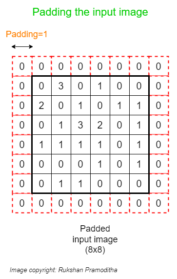
After applying Padding, the new size of the input image is (8, 8). If we do the convolution operation now with Stride=1, we get a feature map of size (6x6) that is equal to the size of the original image before applying Padding.

The above diagrams show the convolution operation with a grayscale image and a single filter. You should also have an idea of the convolution operation when the image is RGB and there are multiple filters involved in the process.

Convolution operation with multiple filters

Here, I only changed the number of filters. The input image type is still grayscale.

The only difference is that another dimension is added to the feature map. It is the third dimension which denotes the number of filters.

Convolution operation on an RGB image

Here, I apply convolution operation on an RGB image. A single filter is used here.

When the image is RGB, the filter should have 3 channels. This is because an RGB image has 3 color channels and 3-channel filters are needed to do the calculations.

Here, the calculation happens on each corresponding channel between the image section and the filter as previously. The final result is obtained by adding all outputs of each channel's calculations. That’s why the feature map does not have a third dimension.

Convolution operation on an RGB image with multiple filters

This is the most complicated version and also the real-world scenario.

Here also, another dimension is added to the feature map. It is the third dimension which denotes the number of filters.

Pooling layers and pooling operation

Pooling layers are the second type of layer used in a CNN. There can be multiple pooling layers in a CNN. Each convolutional layer is followed by a pooling layer. So, convolution and pooling layers are used together as pairs.

Objectives:

• Extract the most important (relevant) features by getting the maximum number or averaging the numbers.
• Reduce the dimensionality (number of pixels) of the output returned from previous convolutional layers.
• Reduce the number of parameters in the network.
• Remove any noise present in the features extracted by previous convolutional layers.
• Increase the accuracy of CNNs.

There are three elements in the pooling layer: Feature map, Filter and Pooled feature map. The pooling operation occurs in each pooling layer.

The pooling operation happens between a section of the feature map and the filter. It outputs the pooled feature map.

There are two types of pooling operations.

• Max pooling: Get the maximum value in the area where the filter is applied.
• Average pooling: Get the average of the values in the area where the filter is applied.

The following diagram shows the max pooling operation applied on the feature map obtained from the previous convolution operation.

Filter: This time, the filter is just a window as there are no elements inside it. So, there are no parameters to learn in the pooling layer. The filter is just used to specify a section in the feature map. The size of the filter should be specified by the user as a hyperparameter. The size should be smaller than the size of the feature map. If the feature map has multiple channels, we should use a filter with the same number of channels. The pooling operations will be done on each channel independently.

Feature map section: The size of the feature map section should be equal to the size of the filter we choose. We can move the filter vertically and horizontally on the feature map to create different sections. The number of sections depends on the Stride we use.

Pooled feature map: The pooled feature map stores the outputs of different pooling operations between different feature map sections and the filter. This will be the input for the next convolution layer (if any) or for the flatten operation.

Stride and padding in the pooling operation

• Stride: Here, the Stride is usually equal to the size of the filter. If the filter size is (2x2), we use Stride=2.
• Padding: Padding is applied to the feature map to adjust the size of the pooled feature map.

Both Stride and Padding are hyperparameters that we need to specify in the pooling layer.

Note: After applying pooling to the feature map, the number of channels is not changed. It means that we have the same number of channels in the feature map and the pooled feature map. If the feature map has multiple channels, we should use a filter with the same number of channels. The pooling operations will be done on each channel independently.

Flatten operation

In a CNN, the output returned from the final pooling layer (i.e. the final pooled feature map) is fed to a Multilayer Perceptron (MLP) that can classify the final pooled feature map into a class label.

An MLP only accepts one-dimensional data. So, we need to flatten the final pooled feature map into a single column that holds the input data for the MLP.

Unlike flattening the original image, important pixel dependencies are retained when pooled maps are flattened.

The following diagram shows how we can flatten a pooled feature map that contains only one channel.

The following diagram shows how we can flatten a pooled feature map that contains multiple channels.

Fully connected (dense) layers

These are the final layers in a CNN. The input is the previous flattened layer. There can be multiple fully connected layers. The final layer does the classification (or other relevant) task. An activation function is used in each fully connected layer.

Objectives:

• Classify the detected features in the image into a class label.

Layer arrangement in a CNN

Here, I discuss how each layer is added to make the entire CNN architecture. In a typical CNN, the layers are arranged in the following order.

A CNN input takes the image as it is. The input image goes through a series of layers and operations.

Convolutional and pooling layers are needed to extract the features from the image while maintaining the important pixel dependencies. They also reduce the dimensionality (number of pixels) in the original image. These layers are used together as pairs.

The ReLU activation is used in each convolutional layer.

The number of filters increases in each convolutional layer. For example, if we use 16 filters in the first convolutional layer, we usually use 32 filters in the next convolutional layer, and so on.

The first few layers focus on less important patterns (such as edges) in the image data. The end layers find more complex patterns (e.g. nose, eyes in a face image). The final layer makes the classification task.

The ReLU activation is used in each fully connected layer except in the final layer in which we use the Softmax activation for multiclass classification.

By looking at the above diagram, we can think of a CNN as a modified version of an MLP. The layers in the green box make some modifications to the image. The orange box contains the MLP. There is the flattened layer between the green box and the orange box.

Note: The coding part of layer arrangement in a CNN will be done with Keras in a separate article.

This is the end of today’s post.

Please let me know if you’ve any questions or feedback.

I hope you enjoyed reading this article. If you’d like to support me as a writer, kindly consider signing up for a membership to get unlimited access to Medium. It only costs $5 per month and I will receive a portion of your membership fee.

Thank you so much for your continuous support! See you in the next article. Happy learning to everyone!

Join my neural network and deep learning course

Rukshan Pramoditha 2022–06–20