Confidence Intervals vs Prediction Intervals

Confusing the two can be costly. See how they differ and when to use each!

Both confidence intervals and prediction intervals express uncertainty in statistical estimates. However, each pertains to uncertainty coming from a different source. Sometimes, one can calculate both for the same quantity, which leads to confusion and potentially grave mistakes in interpreting statistical models. Let’s see how they differ, what uncertainties they express, and when to use each.

Uncertainty intervals in regression models

Let’s start practically by fitting a simple linear regression model to California housing data. We will use only the first 200 records and skip the first one as a test case. The model predicts the house value based on a single predictor, the median income in the neighborhood. We are using only one predictor to be able to easily see the regression line in 2D.

In the model summary, we see the following table.

===========================================================
          coef  std err       t   P>|t   [0.025    0.975]
-----------------------------------------------------------
const   0.7548    0.078   9.633   0.000   0.600   0.909
MedInc  0.3813    0.021  18.160   0.000   0.340   0.423

The coefficient of the median neighborhood income, MedInc, is 0.3813 with a 95% interval around it amounting to 0.340 — 0.423. This is a confidence interval. Confidence interval pertains to a statistic estimated from multiple values, in this case — the regression coefficient. It expresses sampling uncertainty, which comes from the fact that our data is just a random sample of the population we try to model. It can be interpreted as follows: if we had collected many other data sets on houses in California and had fit such a model to each of them, in 95% of the cases the true population coefficient (which we would know should we have data on all houses in California) would fall within the confidence interval.

Confidence interval pertains to a statistic estimated from multiple values. It expresses sampling uncertainty.

Now, let’s use the model to make a prediction for the first observation we have left out from training. Instead of the predict() method, we will use get_predict() combined with summary_frame() in order to extract some more information about the predictions.

We get the following data frame:

  mean mean_se mean_ci_lower mean_ci_upper obs_ci_lower obs_ci_upper
3.9295  0.1174      3.697902      4.161218     2.711407     5.147713

The predicted value for this particular house is 3.9295. Now, the mean_ci columns contain the lower and upper bounds of the confidence interval for this prediction, while the obs_ci columns contain the lower and upper bounds of the prediction interval for the prediction.

You can immediately see that the prediction interval is much wider than the confidence interval. We can visualize it nicely by using the model to predict house values for a range of different neighborhood incomes so that we can see the regression line and the intervals around the predicted values.

Now, pred is just like before, only with 500 rows, and contains predictions and interval bounds for 500 different income values ranging between 0 and 15. We can now use it to plot the regression line and the intervals around it.

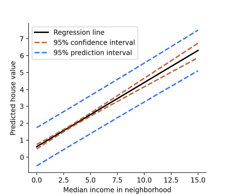
There are two main things to see here. First, the confidence interval is thinner for median income values of 2 through 5 and wider at more extreme values. This is because, for most records in the data, the income is somewhere between 2 and 5. For such cases, the model has more data, hence the sampling uncertainty is smaller.

Second, the prediction interval is much wider than the confidence interval. This is because expresses more uncertainty. On top of the sampling uncertainty, the prediction interval also expresses inherent uncertainty in the particular data point.

Prediction interval expresses inherent uncertainty in the particular data point on top of the sampling uncertainty. Is it thus wider than the confidence interval.

This data-point-level uncertainty comes from the fact that there could be multiple houses of different values in the same neighborhood, and hence with the same predictor value in the model. This is obvious in this particular example, but can also be true in other cases. It happens that multiple feature vectors that are very similar or even exactly the same are associated with different target values.

Let’s recap:

• Confidence intervals express sampling uncertainty in quantities estimated from many data points. The more data, the less sampling uncertainty, and hence the thinner the interval.
• Prediction intervals, on top of the sampling uncertainty, also express uncertainty around a single value, which makes them wider than the confidence intervals.

But where do these intervals come from, and how come they encompass these different sources of uncertainty? Let’s take a look at it next!

Where intervals come from

In old-school statistics, one would calculate the intervals around the prediction y-hat as

where t-crit is the critical value from the t-distribution and SE is the standard error of prediction. Both numbers on the right-hand side will be different for the confidence interval and for the prediction interval and are computed based on various assumptions.

The times of parametric assumptions in statistics, however, are luckily coming to an end. The recent increase in computing power allows for using simple, one-size-fits-all resampling methods to do statistics. Hence, instead of boring you with derivations and formulas, let me show you how to construct both types of intervals via resampling. This approach is applicable not only to linear regression but essentially to any machine learning model you can think of. Moreover, it will make it instantaneously clear what kind of uncertainty is covered by which interval.

Bootstrapping

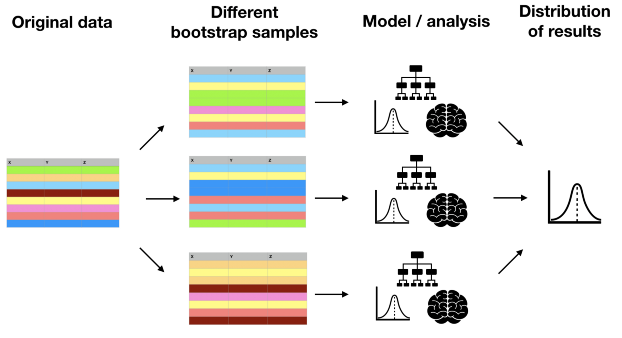
The resampling technique we will use is bootstrapping. It boils down to taking many, say 10 000, samples from the original data with replacement. These are called bootstrap samples, and since we are drawing with replacement, the same observation may appear multiple times in a single bootstrap sample. The point of this is to get many samples from a hypothetical population so that we can observe sampling uncertainty. Next, we perform whatever analysis or model we want on each bootstrap sample separately and compute a quantity of interest, such as a model parameter or a single prediction. Once we have 10 000 bootstrapped values for this quantity, we can look at the percentiles to get the intervals. The entire process is illustrated by the diagram below.

Bootstrapping confidence intervals

Let’s bootstrap confidence intervals for a house value prediction for a house located in the neighborhood with a median income of 3. We take 10 000 bootstrap samples, fit a regression model to each of them, and make a prediction for MedInc equal to 3. This way, we got 10 000 predictions. We can print their mean, and the percentiles denoting the lower and upper bound of the confidence interval.

Mean pred: 1.9019164610645232
95% CI: [1.83355697 1.97350956]

This bootstrap sample accounts for the sampling uncertainty, and so the interval we got is a confidence interval. Let’s now look at how to bootstrap a prediction interval.

Bootstrapping prediction intervals

Prediction interval, on top of the sampling uncertainty, should also account for the uncertainty in the particular prediction data point. To do this, we need one small change in the code. Once we obtain the prediction from the model, we also draw a random residual from the model and add it to this prediction. This way, we can include the individual prediction uncertainty in the bootstrap output.

Mean pred: 1.9014631013163406
95% PI: [1.07444778 2.72920388]

As expected, the prediction interval is significantly wider than the confidence interval, even though the mean prediction is the same.

Thanks for reading!

If you liked this post, why don’t you subscribe for email updates on my new articles? And by becoming a Medium member, you can support my writing and get unlimited access to all stories by other authors and yours truly.

Want to always keep your finger on the pulse of the increasingly faster-developing field of machine learning and AI? Check out my new newsletter, AI Pulse. Need consulting? You can ask me anything or book me for a 1:1 here.

You can also try one of my other articles. Can’t choose? Pick one of these: