Computer Vision 101: Working with Color Images in Python

Learn the basics of working with RGB and Lab images to boost your computer vision projects!

Every computer vision project — be it a cat/dog classifier or bringing colors to old images/movies — involves working with images. And in the end, the model can only be as good as the underlying data — garbage in, garbage out. That is why in this post I focus on explaining the basics of working with color images in Python, how they are represented and how to convert the images from one color representation to another.

Setup

In this section, we set up the Python environment. First, we import all the required libraries:

import numpy as np

from skimage.color import rgb2lab, rgb2gray, lab2rgb
from skimage.io import imread, imshow

import matplotlib.pyplot as plt

We use scikit-image, which is a library from scikit-learn’s family that focuses on working with images. There are many alternative approaches, some of the libraries include matplotlib, numpy, OpenCV, Pillow, etc.

In the second step, we define a helper function for printing out a summary of information about the image — its shape and the range of values in each of the layers.

The logic of the function is pretty straightforward, and the slicing of dimensions will make sense as soon as we describe how the images are stored.

Grayscale

We start with the most basic case possible, a grayscale image. Such images are made exclusively of shades of gray. The extremes are black (weakest intensity of contrast) and white (strongest intensity).

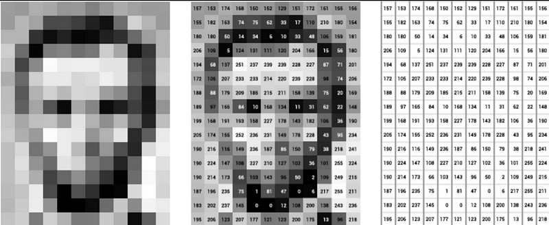
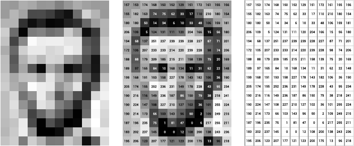
Under the hood, the images are stored as a matrix of integers, in which a pixel’s value corresponds to the given shade of gray. The scale of values for grayscale images ranges from 0 (black) to 255 (white). The illustration below provides an intuitive overview of the concept.

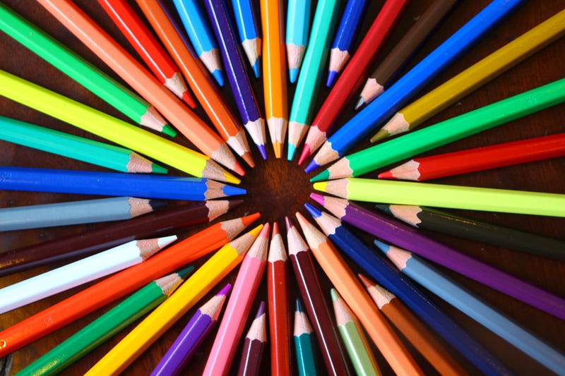
In this article, we will be working with the image you already saw as the thumbnail, the circle of colorful crayons. It was not accidental that such a colorful picture was selected :)

We start by loading the grayscale image into Python and printing it.

image_gs = imread('crayons.jpg', as_gray=True)

fig, ax = plt.subplots(figsize=(9, 16))
imshow(image_gs, ax=ax)
ax.set_title('Grayscale image')
ax.axis('off');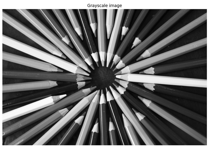

As the original image is in color, we used as_gray=True to load it as a grayscale image. Alternatively, we could have loaded the image using the default settings of imread (which loads an RGB image — covered in the next section) and converted it to grayscale using the rgb2gray function.

Next, we run the helper function to print the summary of the image.

print_image_summary(image_gs, ['G'])

Running the code produces the following output:

--------------
Image Details:
--------------
Image dimensions: (1280, 1920)
Channels:
G : min=0.0123, max=1.0000

The image is stored as a 2D matrix, 1280 rows by 1920 columns (high-definition resolution). By looking at the min and max values, we can see that they are in the [0,1] range. That is because they were automatically divided by 255, which is a common preprocessing step for working with images.

RGB

Now it is time to work with colors. We start with the RGB model. In short, it is an additive model, in which shades of red, green and blue (hence the name) are added together in various proportions to reproduce a broad spectrum of colors.

In scikit-image, this is the default model for loading the images using imread:

image_rgb = imread('crayons.jpg')

Before printing the images, let’s inspect the summary to understand the way the image is stored in Python.

print_image_summary(image_rgb, ['R', 'G', 'B'])

Running the code generates the following summary:

--------------
Image Details:
--------------
Image dimensions: (1280, 1920, 3)
Channels:
R : min=0.0000, max=255.0000
G : min=0.0000, max=255.0000
B : min=0.0000, max=255.0000

In comparison to the grayscale image, this time the image is stored as a 3D np.ndarray. The additional dimension represents each of the 3 color channels. As before, the intensity of the color is presented on a 0–255 scale. It is frequently rescaled to the [0,1] range. Then, a pixel’s value of 0 in any of the layers indicates that there is no color in that particular channel for that pixel.

A helpful note: When using the OpenCV’s imread function, the image is loaded as BGR instead of RGB. To make it compatible with other libraries, we need to change the order of the channels.

It is time to print the image and the different color channels:

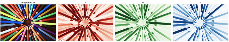
fig, ax = plt.subplots(1, 4, figsize = (18, 30))

ax[0].imshow(image_rgb/255.0) 
ax[0].axis('off')
ax[0].set_title('original RGB')

for i, lab in enumerate(['R','G','B'], 1):
    temp = np.zeros(image_rgb.shape)
    temp[:,:,i - 1] = image_rgb[:,:,i - 1]
    ax[i].imshow(temp/255.0) 
    ax[i].axis("off")
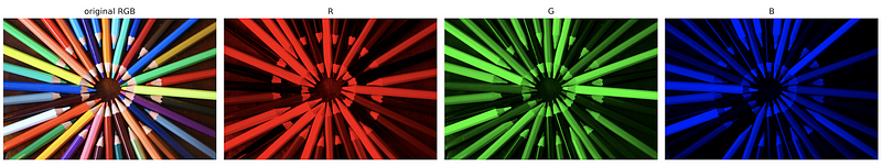
    ax[i].set_title(lab)

plt.show()

In the image below, we can see the original image and the 3 color channels separately. What I like about this image is that by focusing on individual crayons, we can see which colors from the RGB channels and in which proportions constitute the final color in the original image.

Alternatively, we can plot the separate color channels as follows:

fig, ax = plt.subplots(1, 4, figsize = (18, 30))

ax[0].imshow(image_rgb) 
ax[0].axis('off')
ax[0].set_title('original RGB')

for i, cmap in enumerate(['Reds','Greens','Blues']):
    ax[i+1].imshow(image_rgb[:,:,i], cmap=cmap) 
    ax[i+1].axis('off')
    ax[i+1].set_title(cmap[0])

plt.show()

What generates the following output:

What I prefer about this variant of plotting the RGB channels is that I find it easier to distinguish the different colors (they stand out more due to the others being much lighter and transparent) and their intensity.

We can often encounter RGB images while working on image classification tasks. When applying convolutional neural networks (CNNs) for that task, we need to apply all the operations to all 3 color channels. In this article, I show how to use CNNs to work with a binary image classification problem.

Lab

Next to RGB, another popular way of representing color images is with the Lab color space (also knows as CIELAB).

Before going into more detail, it makes sense to point out the difference between a color model and a color space. A color model is a mathematical way of describing colors. A color space is the method of mapping real, observable colors to the color model’s discrete values. For more details please refer to this answer.

The Lab color space expresses colors as three values:

• L: the lightness on a scale from 0 (black) to 100 (white), which in fact is a grayscale image
• a: green-red color spectrum, with values ranging from -128 (green) to 127 (red)
• b: blue-yellow color spectrum, with values ranging from -128 (blue) to 127 (yellow)

In other words, Lab encodes an image into a grayscale layer and reduces three color layers into two.

We start by converting the image from RGB to Lab and printing the image summary:

image_lab = rgb2lab(image_rgb / 255)

The rgb2lab function assumes that the RGB is standardized to values between 0 and 1, that is why divided all the values by 255. From the following summary, we see that the range of Lab values falls within the ones specified above.

--------------
Image Details:
--------------
Image dimensions: (1280, 1920, 3)
Channels:
L : min=0.8618, max=100.0000
a : min=-73.6517, max=82.9795
b : min=-94.7288, max=91.2710

As the next step, we visualize the image — the Lab one and each of the channels separately.

fig, ax = plt.subplots(1, 4, figsize = (18, 30))

ax[0].imshow(image_lab) 
ax[0].axis('off')
ax[0].set_title('Lab')

for i, col in enumerate(['L', 'a', 'b'], 1):
    imshow(image_lab[:, :, i-1], ax=ax[i])
    ax[i].axis('off')
    ax[i].set_title(col)

fig.show()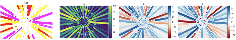

Well, the 1st attempt to visualizing the Lab color space was far from successful. The first image is close to unrecognizable, the L layer is not grayscale. Following the insights from this answer, in order to be printed correctly, the Lab values must be rescaled to the [0,1] range. This time, the first layer is rescaled differently than the latter two.

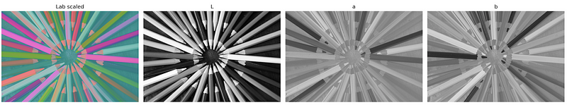
#scale the lab image
image_lab_scaled = (image_lab + [0, 128, 128]) / [100, 255, 255]

fig, ax = plt.subplots(1, 4, figsize = (18, 30))

ax[0].imshow(image_lab_scaled) 
ax[0].axis('off')
ax[0].set_title('Lab scaled')

for i, col in enumerate(['L', 'a', 'b'], 1):
    imshow(image_lab_scaled[:, :, i-1], ax=ax[i])
    ax[i].axis('off')
    ax[i].set_title(col)
    
fig.show()

The second attempt is much better. In the first image, we see the Lab representation of the color image. This time, the L layer is an actual grayscale image. What could still be improved are the last two layers, as they are in grayscale as well.

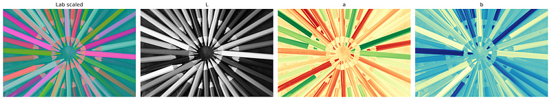
In the last attempt, we apply color maps to the a and b layers of the Lab image.

fig, ax = plt.subplots(1, 4, figsize = (18, 30))

ax[0].imshow(image_lab_scaled) 
ax[0].axis('off')
ax[0].set_title('Lab scaled')

imshow(image_lab_scaled[:,:,0], ax=ax[1]) 
ax[1].axis('off')
ax[1].set_title('L')

ax[2].imshow(image_lab_scaled[:,:,1], cmap='RdYlGn_r') 
ax[2].axis('off')
ax[2].set_title('a')

ax[3].imshow(image_lab_scaled[:,:,2], cmap='YlGnBu_r') 
ax[3].axis('off')
ax[3].set_title('b')
    
plt.show()

This time the results are satisfactory. We can clearly distinguish different colors in the a and b layers. What could still be improved are the colormaps themselves. For simplicity, I used the predefined color maps, which contain a color in-between the two extreme ones (yellow for layer a, green in the b layer). A potential solution is to code the color maps manually.

Lab images are commonly encountered while working with image colorization problems, such as the famous DeOldify.

Conclusions

In this article, I went over the basics of working with color images in Python. Using the presented techniques, you can start working on a computer vision problem on your own. I believe it is important to understand how the images are stored and how to transform them into different representations, so that you do not run into unexpected problems while training deep neural networks.

Another popular color space is the XYZ. scikit-image also contains functions for converting RGB or Lab images into XYZ.

You can find the code used for this article on my GitHub. As always, any constructive feedback is welcome. You can reach out to me on Twitter or in the comments.

I recently published a book on using Python for solving practical tasks in the financial domain. If you are interested, I posted an article introducing the contents of the book. You can get the book on Amazon or Packt’s website.

References

[1] https://ai.stanford.edu/~syyeung/cvweb/tutorial1.html

[2] https://github.com/scikit-image/scikit-image/issues/1185