Comprehensive Cheat Sheet for Python Pandas

The most common Pandas functions for data wrangling

Undoubtedly Pandas is one of the most popular Python libraries for data science. Its versatility and functionalities make it a powerful tool for data wrangling and exploration. Getting familiar with Pandas has become an essential skill for data science professionals.

In this article, we will discuss common Pandas functions for data wrangling. Hopefully, this would be a helpful cheat sheet when using Pandas.

Import Data from an Existing Data Source

Import a CSV file

df = pd.read_csv('file_name.csv')

Import an Excel file

df = pd.read_excel(open('file_name.xlsx', 'rb'), sheet_name='sheet_name')

Import a file from a website

df = pd.read_csv('https://archive.ics.uci.edu/ml/machine-learning-databases/iris/iris.data')

Import data from a SQL Database

Before we write a query to pull data from a SQL Database, we need to connect to the database with a valid credential. SQLAlchemy makes it easy to interact between Python and SQL Database.

import sqlalchemy

connection = sqlalchemy.create_engine('dialect+driver://username:password@host:port/database').connect()

sql = 'CREATE TABLE df AS SELECT ...'
connection.execute(sql)

df = pd.read_sql('SELECT * FROM df', con=connection)

Create DataFrame

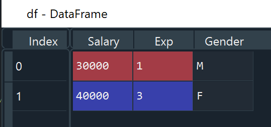
Method 1: Create DataFrame from a list of dictionaries

data = [{'Salary': 30000, 'Exp': 1, 'Gender': 'M'},             
        {'Salary': 40000, 'Exp': 3, 'Gender': 'F'}]        
df = pd.DataFrame(data)

Output:

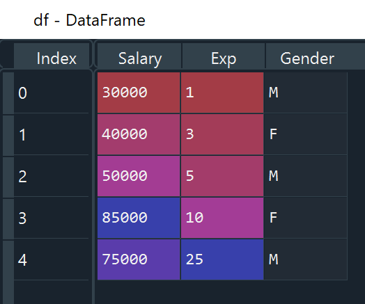
Method 2: Create DataFrame from a dictionary of lists

data= {'Salary': [30000, 40000, 50000, 85000, 75000],            
        'Exp': [1, 3, 5, 10, 25],          
        'Gender': ['M','F', 'M', 'F', 'M']} 
df = pd.DataFrame(data)

Output:

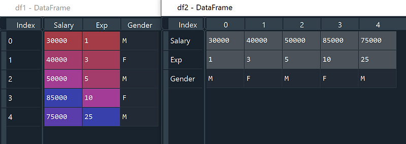
Method 3: Create DataFrame using from_dict. If you would like to use the keys of the passed dict as the column names of the resulting DataFrame, set orient to be ‘columns’. Otherwise, if the keys should be rows, set orient to be ‘index’.

data= {'Salary': [30000, 40000, 50000, 85000, 75000],            
        'Exp': [1, 3, 5, 10, 25],          
        'Gender': ['M','F', 'M', 'F', 'M']} 
df1 = pd.DataFrame.from_dict(data, orient = 'columns')
df2 = pd.DataFrame.from_dict(data, orient = 'index')

Output:

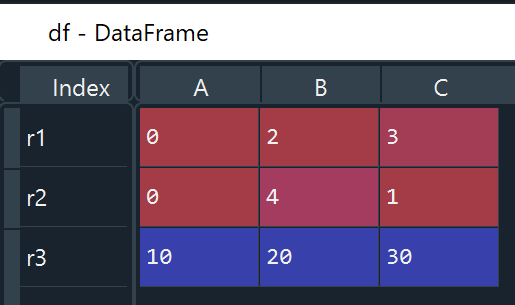
Method 4: Create DataFrame from a list of multiple lists. We can have user-defined indexes and column names using “index” and “columns” options respectively.

# pd.DataFrame([[Row 1], [Row 2], [Row 3],...])
df = pd.DataFrame([[0, 2, 3], [0, 4, 1], [10, 20, 30]],                   index=['r1', 'r2', 'r3'], columns=['A', 'B', 'C'])

Output:

Preview DataFrame

head & tail: These two functions return the first n and last n rows of a dataframe respectively.

# Return the first 5 observations of a dataframe
df.head(5)

# Return the last 5 observations of a dataframe
df.tail(5)

Trick: When previewing a huge CSV file (>10GB), a quick snippet of data could be very helpful to determine the information in the data file and its data structure. We can use skiprows and nrows options in read_csv to specify the number of lines we want to skip and read, which might reduce importing time from hours to a few seconds.

preview_df = pd.read_csv('Big_data.csv', skiprows = 0, nrows = 100, header=0, engine='python')

columns & info: columns and info functions could output column names and the data type of each column.

df.columns
df.info()

Trick: We can use value_counts to output counts of unique values for a given column. Sometimes, we need to produce a cross-tabulation of two columns. crosstab is a handy function to serve that purpose.

df['City'].value_counts()
Out[19]: 
Yangon       340
Mandalay     332
Naypyitaw    328
Name: City, dtype: int64

pd.crosstab(df['Product line'], df['City'])
Out[22]: 
City                    Mandalay  Naypyitaw  Yangon
Product line                                       
Electronic accessories        55         55      60
Fashion accessories           62         65      51
Food and beverages            50         66      58
Health and beauty             53         52      47
Home and lifestyle            50         45      65
Sports and travel             62         45      59

describe: This function outputs a descriptive statistical summary that includes the number of observations, mean, standard deviation, min, max, and percentiles.

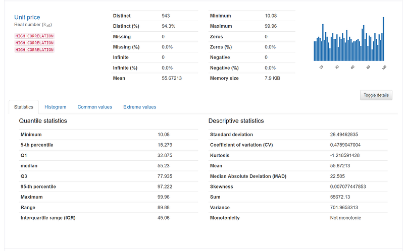
df.describe()

Trick: Similar to describe, pandas_profiling.ProfileReport can produce basic information and a descriptive statistical summary of each column. It also generates a comprehensive data exploration report

# Install the library
!pip install pandas-profiling

# Import the library
import pandas_profiling

profile = pandas_profiling.ProfileReport(df, title = "Data Exploration")
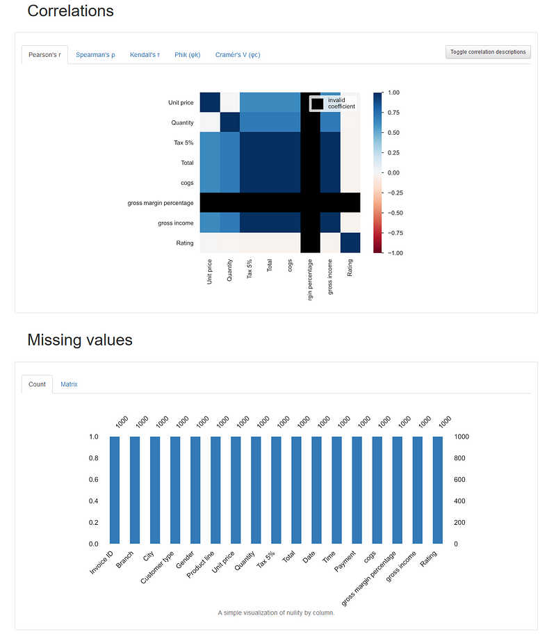
profile.to_file(output_file='Data Profile Output.html')

It produces a quick histogram of each column and allows us to create a scatter plot of any two numeric columns. Moreover, it also includes correlations of columns and counts of missing values.

Subset DataFrame

Let’s create a dataframe, which includes an index of [‘r1’, ‘r2’, ‘r3’] and columns of [‘A’, ‘B’, ‘C’].

# Create a dataframe
df2 = pd.DataFrame([[0, 2, 3], [0, 4, 1], [10, 20, 30]],                 index=['r1', 'r2', 'r3'], columns=['A', 'B', 'C'])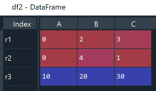

Row Selection Using Bracket

df[Beginning Row : Ending Row]: This would give a subset of consecutive rows of data. For example, df2[0:3] produces the first row to the third row in a dataframe.

Trick: df2[0] doesn’t extract the first row. Instead, this would give us a column with a name of “0”, which is not available in our data columns, [‘A’, ‘B’, ‘C’]. Instead, we should use df[0:1] to get the first row.

df[condition(boolean)]: This would create a subset of dataframe based on a boolean condition. For example, df2[df2[‘C’] > 10] produces rows where column “C” is greater than 10.

Trick: We can also use query to specify a boolean expression. Using querywe don’t need to explicitly write dataframe name multiple times.

# df[df['Gender']=='Female']
df.query('Gender == "Female"')

# df[df['Quantity']> 7]
df.query('Quantity > 7')

Row Selection Using iloc

df.iloc[Selected Row(s),:]: iloc allows us to extract a subset based on row numbers. For example: df2.iloc[0:10, :] would produce the first 10 rows and df2.iloc[[0, 2, 5], :] would produce a subset that contains the first, third and sixth rows. The : inside the square bracket implies that we would keep all the columns.

Row Selection Using loc

df.loc[Selected Index, :]: loc allows a user to extract a subset based on an index. For example, df2.loc[‘r1’, :] would produce a subset with “index = ‘r1’”. df2.loc[[‘r1’, ‘r2’],:] would produce a subset with “index = ‘r1’ and ‘r2’”.

Column Selection Using Double Bracket

df[[Selected Columns]]: With a double bracket, we can select single or multiple columns in a dataframe. For example, df[[‘Unit price’, ‘Quantity’]] would extract ‘Unit price’ and ‘Quantity’ columns in the dataframe.

Trick: Single Bracket vs Double Bracket. We can use a single bracket to extract a single column. But the output will be stored as a series, whereas a double bracket would give us a dataframe.

test1 = df[['Quantity']]

type(test1)
Out[176]: pandas.core.frame.DataFrame

test2 = df['Quantity']

type(test2)
Out[178]: pandas.core.series.Series

df.iloc[:, Selected Column Numbers] vs df.loc[:, Selected Column Names]: Both iloc and loc can extract a subset of columns from a dataframe. The difference is iloc is based on the column number, whereas loc is using the actual column name. For example, df2.iloc[:, 0] would extract the first column without mentioning the column name, and df2.loc[:, ‘A’] would extract column “A” from the dataframe.

Window Functions

Window Functions are implemented on a set of rows called a window frame. A window frame is all the rows within the same group based on one or more columns. When a window function is implemented, a new column would be produced and the output would have the same number of rows as the original data set.

Create a New Column of Row number

df.groupby('gender')['{any column name}'].rank('first')
# or
df.groupby('gender').cumcount()+1

Create Count/Max/Min/Average/Sum Within a Group

In Pandas, we often use transform with a window function, such as, count, max, min, avg and sum.

df.groupby('gender')['salary'].transform('count')
df.groupby('gender')['salary'].transform('max')
df.groupby('gender')['salary'].transform('min')
df.groupby('gender')['salary'].transform('mean')
df.groupby('gender')['salary'].transform('sum')

Create Running Sum Within a Group

df.groupby('gender')['salary'].transform('cumsum')

Create Percentiles Within a Group

# create median 
df.groupby('gender')['salary'].transform(lambda x: x.quantile(0.5))

Create Lag/Lead Within a Group

# create lag variable
df.groupby('gender')['salary'].transform(lambda x: x.shift(1)) 
# create lead variable
df.groupby('gender')['salary'].transform(lambda x: x.shift(-1))

Create Ranking Within a Group

df.groupby('gender')['salary'].rank('dense', ascending = False) # e.g., 1,2,2,3, ...
df.groupby('gender')['salary'].rank('min', ascending = False) # e.g., 1,2,2,4, ...

Aggregate Functions

Aggregate Functions are implemented in the same as window functions. But the result will be more compact. The number of observations in the final output would equal the number of distinct groups (i.e., unique values in group-by variables).

Collapse Rows With Count/Max/Min/Average/Sum Within a Group

In Pandas, there are many ways to implement an aggregate function. I include 3 different ways in the following code snippet.

• An aggregate function would run as the default using groupby
• Use apply to run a built-in aggregate function or a user-defined function with groupby
• Use agg to run a built-in aggregate function or a user-defined function with more flexibility, such as, naming new columns and creating more than one new column

df.groupby('gender')['salary'].mean().reset_index()
df.groupby('gender')['salary'].min().reset_index()
df.groupby('gender')['salary'].max().reset_index()
df.groupby('gender')['salary'].sum().reset_index()

df.groupby('gender').apply(lambda x: x['salary'].mean()).reset_index()

df.groupby('gender').agg(count = pd.NamedAgg('salary', 'mean')).reset_index()

Create Percentile Within a Group

df.groupby(‘gender’)[‘salary’].quantile(0.9).reset_index()

Missing Values

We’ll use the following dataframe to discuss how to handle missing values.

data = {'emp_id': [1, 1, 2, 2],
        'emp_name': ['Jane Dow', 'Jane Dow', 'Thomas Daley', 'Thomas Daley'],
        'gender': [np.nan, 'M', 'F', 'F'],
        'year': [2019, 2020, 2019, 2020],
        'compensation': [53000, np.nan, 53000, '$56,000']}

df2  = pd.DataFrame(data)
df2

Out[107]: 
   emp_id      emp_name gender  year compensation
0       1      Jane Dow    NaN  2019        53000
1       1      Jane Dow      M  2020          NaN
2       2  Thomas Daley      F  2019        53000
3       2  Thomas Daley      F  2020      $56,000

isnull() & notnull(): isnull() allows us to display rows with missing values based on a specified column, whereas notnull() would return rows with non-missing values.

df2[df2['compensation'].isnull()]
Out[108]: 
   emp_id  emp_name gender  year compensation
1       1  Jane Dow      M  2020          NaN

df2[df2['compensation'].notnull()]
Out[109]: 
   emp_id      emp_name gender  year compensation
0       1      Jane Dow    NaN  2019        53000
2       2  Thomas Daley      F  2019        53000
3       2  Thomas Daley      F  2020      $56,000

fillna(): it allows us to replace the missing value with any value. In this case, we replace missing compensation with the value of 0. (You can check out my other article discussing Missing Data.)

df2['compensation'].fillna(0, inplace = True)

String Operation

str.split(): it allows us to split text in a given column into multiple columns. In the following code, “emp_name” column is split into “first_name” and “last_name” columns using the option expand = True. By default, text in a column is split by whitespace, but you can specify the separator using the option pat = '<str>' .

df2[['first_name', 'last_name']] = df2['emp_name'].str.split(expand = True)
print(df2)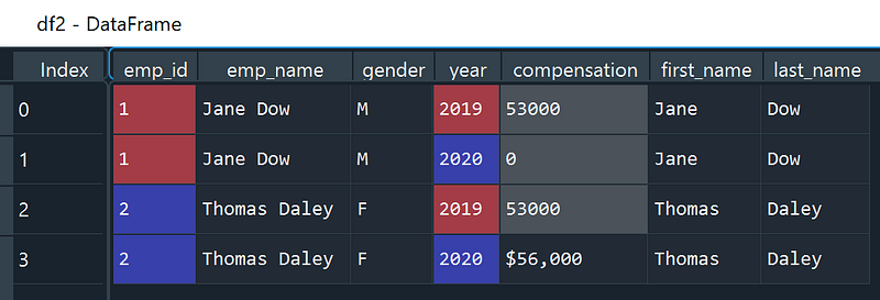

str.replace & re.sub(): It is tempting to just use str.replace() to remove “$” and “,”. But when we do that, we notice that the integer values would be replaced with np.nan since str.replace() doesn’t work with integer values.

# Incorrect Method 
df2['compensation'].str.replace('\$|,', '')

Out[124]: 
0      NaN
1      NaN
2      NaN
3    56000
Name: compensation, dtype: object

Trick: To correctly clean a column with a mix of string and numeric values, we need to first convert values in the column into string values using astype() , then use either str.replace() or re.sub() to replace the relevant string values as needed. Lastly, we convert the column back to numeric values.

# Method 1: Using str.replace() with astype()
df2['compensation'].astype(str).str.replace('\$|,', '').astype(int)

# Method 2: Using apply with re.sub()
df2['compensation'] = df2.apply(lambda x: re.sub('\$|,', '', str(x['compensation'])), axis = 1).astype(int)

Join Multiple DataFrames

Combining Rows

append() & concat(): We can use either append() or concat() to combine two dataframes in a row-wise fashion. Then we can use reset_index(drop=True) to reset the index in the combined dataframe.

df.append(df2).reset_index(drop=True)
pd.concat([df, df2]).reset_index(drop=True)

Combining Columns

join() & merge(): Both join() or merge() can combine two dataframes in a column-wise fashion. The difference is using join() observations with the same index would be put in the same row, whereas, using merge() the observations with the same values based on the common column(s) would be put in the same row.

df.join(df2)
df2.merge(df5, on = '[Common Columns]', how = [‘left’, ‘right’, ‘outer’, ‘inner’, ‘cross’])

Reformat DataFrame

Convert Dataframe from Long to Wide

Both pivot() and pivot_table() would produce a (wide) table that summarizes the data from a more extensive (long) table. The difference is pivot_table() can also incorporate aggregate functions, such as sum, average, max, min and first. In the following example, we try to create separate compensation columns, “2019” and “2020” based on the “year” column.

df2
Out[200]: 
   emp_id      emp_name gender  year compensation
0       1      Jane Dow      M  2019        53000
1       1      Jane Dow      M  2020            0
2       2  Thomas Daley      F  2019        53000
3       2  Thomas Daley      F  2020      $56,000

df_wide = df2.pivot(index = ['emp_id', 'emp_name', 'gender'], columns = ['year'], values = 'compensation').reset_index()
print(df_wide)
year  emp_id      emp_name gender   2019     2020
0          1      Jane Dow      M  53000        0
1          2  Thomas Daley      F  53000  $56,000

df_wide2 = df2.pivot_table(index = ['emp_id', 'emp_name', 'gender'], columns = ['year'], values = 'compensation', aggfunc = 'first').reset_index()
print(df_wide2)
year  emp_id      emp_name gender   2019     2020
0          1      Jane Dow      M  53000        0
1          2  Thomas Daley      F  53000  $56,000

Convert Dataframe from Wide to Long

melt() allows us to change dataframe format from wide to long. This is the opposite of creating a pivot table. In the following example, we want to consolidate compensation columns, “2019” and “2020” into a single column and create a new “year” column.

df_long = df_wide.melt(id_vars= ['emp_id', 'emp_name', 'gender'], var_name= 'year', value_vars= [2019, 2020], value_name="Compensation")
print(df_long)
   emp_id      emp_name gender  year Compensation
0       1      Jane Dow      M  2019        53000
1       2  Thomas Daley      F  2019        53000
2       1      Jane Dow      M  2020            0
3       2  Thomas Daley      F  2020      $56,000

Thank you for reading !!!

If you enjoy this article and would like to Buy Me a Coffee, please click here.

You can sign up for a membership to unlock full access to my articles, and have unlimited access to everything on Medium. Please subscribe if you’d like to get an email notification whenever I post a new article.

More content at PlainEnglish.io. Sign up for our free weekly newsletter. Follow us on Twitter, LinkedIn, YouTube, and Discord. Interested in Growth Hacking? Check out Circuit.