Comprehensive Evaluation of Classification Models: An In-depth Exploration of Confusion Matrix and Derived Metrics

Introduction

The confusion matrix is a critical tool in the field of machine learning and statistics, used to evaluate the performance of classification models. It is a table that allows visualization of the performance of an algorithm, typically a supervised learning one, by comparing the actual and predicted classifications. The matrix helps in understanding how well the classification model is identifying each class. This essay explores the confusion matrix in detail, including its components and the various metrics derived from it, which are instrumental in assessing a model’s performance.

In the world of model evaluation, the confusion matrix is not just a tool; it’s a compass that navigates the sea of data, guiding us toward true understanding and refined accuracy.

Components of the Confusion Matrix

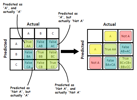
The confusion matrix is composed of four fundamental elements:

1. True Positives (TP): These are the instances correctly predicted as positive by the model.
2. True Negatives (TN): These are the instances correctly predicted as negative by the model.
3. False Positives (FP): These are the instances incorrectly predicted as positive, also known as Type I error.
4. False Negatives (FN): These are the instances incorrectly predicted as negative, also known as Type II error.

These components are used in a matrix format to show the actual class labels against the predicted class labels by the model, providing a detailed breakdown of the model’s predictions.

Metrics Derived from the Confusion Matrix

Various performance metrics can be derived from the confusion matrix, each providing different insights into the model’s performance. These metrics include:

1. Accuracy: It measures the proportion of true results (both true positives and true negatives) in the total data set. It’s calculated as TP+TN​/TP+TN+FP+FN. While accuracy is the most intuitive performance measure, it can be misleading in imbalanced datasets where one class significantly outnumbers the other.
2. Precision (Positive Predictive Value): It measures the proportion of positive identifications that were actually correct. It’s calculated as TP/TP+FP​. Precision is critical in scenarios where the cost of a false positive is high.
3. Recall (Sensitivity, True Positive Rate): It measures the proportion of TP/actual positives that were correctly identified. It’s calculated as TP+FN​. Recall is essential in situations where the cost of a false negative is high.
4. F1 Score: It is the harmonic mean of precision and recall, calculated as 2×Precision×Recall/Precision+Recall. The F1 score is a balanced measure for the test’s accuracy, especially in cases of uneven class distributions.
5. Specificity (True Negative Rate): It measures the proportion of actual negatives that were correctly identified, calculated as TN/TN+FP​. This metric is crucial in situations where it’s important to identify negatives correctly.
6. False Positive Rate: It measures the proportion of actual negatives that were incorrectly identified as positive, calculated as FP​/FP+TN.
7. Negative Predictive Value: It measures the proportion of negative identifications that were actually correct, calculated as TN​/TN+FN.
8. False Discovery Rate: It measures the proportion of positive identifications that were false, calculated as FP/FP+TP​.
9. Matthews Correlation Coefficient (MCC): It provides a comprehensive measure that takes into account true and false positives and negatives, calculated as ​TP×TN−FP×FN/(TP+FP)(TP+FN)(TN+FP)(TN+FN)​. The MCC is considered a balanced measure that can be used even if the classes are of very different sizes.

Code

Creating a synthetic dataset and exploring all possible metrics derived from a confusion matrix involves several steps, including data generation, model training, prediction, and finally, evaluation using the confusion matrix and related metrics. Below is a Python code snippet that covers these aspects, using sklearn for dataset generation and model training, and matplotlib for plotting.

import numpy as np
import matplotlib.pyplot as plt
from sklearn.datasets import make_classification
from sklearn.model_selection import train_test_split
from sklearn.linear_model import LogisticRegression
from sklearn.metrics import (confusion_matrix, accuracy_score, precision_score, 
                             recall_score, f1_score, roc_curve, auc, 
                             precision_recall_curve, average_precision_score, 
                             roc_auc_score, matthews_corrcoef)

# Generate a synthetic binary classification dataset
X, y = make_classification(n_samples=1000, n_features=20, n_classes=2, random_state=42)

# Split dataset into training and testing set
X_train, X_test, y_train, y_test = train_test_split(X, y, test_size=0.3, random_state=42)

# Train a logistic regression model
model = LogisticRegression(solver='liblinear', random_state=42)
model.fit(X_train, y_train)

# Predictions
y_pred = model.predict(X_test)
y_pred_proba = model.predict_proba(X_test)[:, 1]

# Confusion Matrix
cm = confusion_matrix(y_test, y_pred)
print("Confusion Matrix:\n", cm)

# Accuracy, Precision, Recall, F1 Score
accuracy = accuracy_score(y_test, y_pred)
precision = precision_score(y_test, y_pred)
recall = recall_score(y_test, y_pred)
f1 = f1_score(y_test, y_pred)
print(f"Accuracy: {accuracy}\nPrecision: {precision}\nRecall: {recall}\nF1 Score: {f1}")

# ROC Curve and AUC
fpr, tpr, thresholds = roc_curve(y_test, y_pred_proba)
roc_auc = auc(fpr, tpr)

# Plot ROC Curve
plt.figure(figsize=(8, 6))
plt.plot(fpr, tpr, color='darkorange', lw=2, label=f'ROC curve (area = {roc_auc:.2f})')
plt.plot([0, 1], [0, 1], color='navy', lw=2, linestyle='--')
plt.xlim([0.0, 1.0])
plt.ylim([0.0, 1.05])
plt.xlabel('False Positive Rate')
plt.ylabel('True Positive Rate')
plt.title('Receiver Operating Characteristic (ROC) Curve')
plt.legend(loc="lower right")
plt.show()

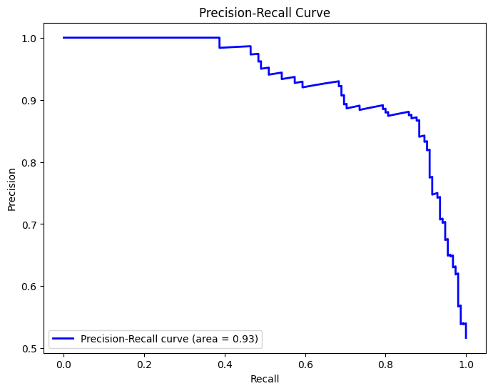
# Precision-Recall Curve and Average Precision
precision, recall, _ = precision_recall_curve(y_test, y_pred_proba)
average_precision = average_precision_score(y_test, y_pred_proba)

# Plot Precision-Recall Curve
plt.figure(figsize=(8, 6))
plt.plot(recall, precision, color='blue', lw=2, label=f'Precision-Recall curve (area = {average_precision:.2f})')
plt.xlabel('Recall')
plt.ylabel('Precision')
plt.title('Precision-Recall Curve')
plt.legend(loc="lower left")
plt.show()

# Matthews Correlation Coefficient
mcc = matthews_corrcoef(y_test, y_pred)
print(f"Matthews Correlation Coefficient: {mcc}")

This code performs the following tasks:

1. Data Generation: Generates a synthetic dataset using make_classification, which is ideal for binary classification tasks.
2. Model Training: Uses LogisticRegression to fit the model on the training data.
3. Prediction: Makes predictions on the test dataset to evaluate the model.
4. Evaluation Metrics: Calculates and prints the confusion matrix, accuracy, precision, recall, F1 score, and Matthews Correlation Coefficient (MCC).
5. ROC Curve: Plots the Receiver Operating Characteristic (ROC) curve along with the Area Under Curve (AUC) to evaluate the model’s performance in distinguishing between the two classes.
6. Precision-Recall Curve: Plots the Precision-Recall curve and calculates the average precision, which is particularly useful in case of imbalanced datasets.

Confusion Matrix:
 [[127  18]
 [ 27 128]]
Accuracy: 0.85
Precision: 0.8767123287671232
Recall: 0.8258064516129032
F1 Score: 0.8504983388704319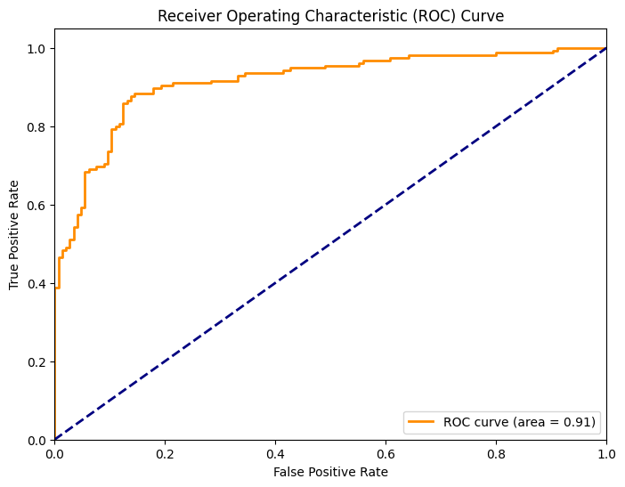

Matthews Correlation Coefficient: 0.7015280729542706

This comprehensive evaluation using a confusion matrix and derived metrics, along with ROC and Precision-Recall curves, provides a detailed insight into the model’s performance on the synthetic dataset.

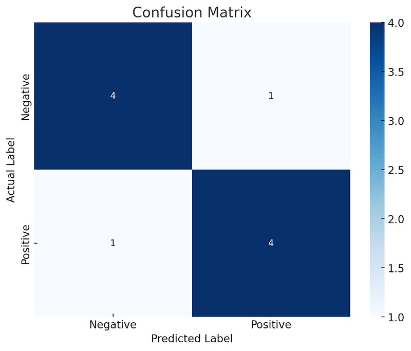
Here’s the plotted confusion matrix, visually representing the performance of the classification model with respect to the actual and predicted labels. The matrix is color-coded for easy interpretation, showing the counts of true positives, true negatives, false positives, and false negatives. This visualization aids in quickly assessing the model’s accuracy and identifying areas for improvement.

Conclusion

The confusion matrix and its derived metrics offer a multifaceted view of a model’s performance, beyond simple accuracy. Each metric provides insights into different aspects of the model’s predictions, such as its precision, recall, and the balance between them (F1 score). Understanding these metrics is crucial for evaluating, comparing, and improving classification models, especially in fields where the cost of false positives or negatives is significant. Through the confusion matrix, data scientists and analysts can identify weaknesses in their models and take steps to address them, ultimately leading to more accurate and reliable predictions.

In Plain English 🚀

Thank you for being a part of the In Plain English community! Before you go:

• Be sure to clap and follow the writer ️👏️️
• Follow us: X | LinkedIn | YouTube | Discord | Newsletter
• Visit our other platforms: Stackademic | CoFeed | Venture | Cubed
• More content at PlainEnglish.io