Summary

The article discusses the concept of cointegration in multivariate time-series analysis, emphasizing the potential pitfalls of differencing when dealing with cointegrated series.

Abstract

The article on cointegrated time-series data delves into the nuances of differencing in multivariate time-series analysis. It contrasts the straightforward application of differencing in univariate time-series with its complex implications in multivariate contexts. The author illustrates this through an artificial two-dimensional linear time-series example, demonstrating that differencing can lead to poorer forecast performance due to cointegration. Cointegration, a phenomenon where a linear combination of non-stationary series is stationary, suggests that the series move together in a long-term equilibrium. The article argues that blindly applying differencing to cointegrated series can result in the loss of valuable information and that alternative approaches, such as incorporating the original series or using error correction models, should be considered. The author advocates for careful analysis and the use of statistical tests, like those developed by MacKinnon, Engle-Granger, and Johansen, to detect cointegration and inform appropriate modeling strategies.

Opinions

The author posits that differencing, while effective for univariate time-series with unit-roots, may not be suitable for multivariate time-series due to cointegration.
It is suggested that the common practice of applying differencing to multivariate data without considering cointegration can lead to suboptimal forecasting models.
The article recommends that practitioners should not automatically difference multivariate time-series data but should instead test for cointegration and adjust their models accordingly.
The author implies that including the original time-series data alongside differenced data could improve model performance in the presence of cointegration.
A pragmatic approach to handling cointegration is endorsed, which involves cross-validation and backtesting to select the most accurate forecasting model.
The author emphasizes the importance of statistical tests for cointegration, highlighting the MacKinnon test and others as essential tools for time-series analysis.
The article concludes by cautioning against the routine application of differencing and encourages further exploration into non-linear cointegration as a next step in research.

Cointegrated time-series and when differencing might be bad

You have heard about integrated time-series data but what about cointegration?

Introduction

A standard method in the time-series analysis toolkit are difference transformations or differencing. Despite being dead simple, differencing can be quite powerful. In fact, it allows us to outperform sophisticated time-series models with what is almost a bare white noise process.

Due to its simplicity, differencing is quite popular whenever some unit-root test is significant. While this is fairly safe in the univariate case, things look differently for multivariate time-series.

Let us demonstrate this with a simple example:

A motivating time-series example

To exemplify the underlying issue, I created an artificial, two-dimensional and linear time-series:

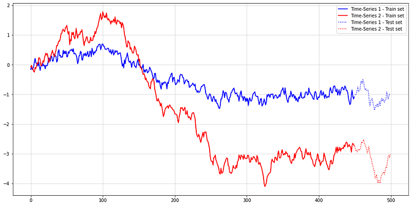
Simple, two-dimensional time-series. (Image by author)

There seems to be some connection between both time-series but that might obviously just be a spurious one over time. The next step that you often see done in this setting is to test for unit-roots in both time-series.

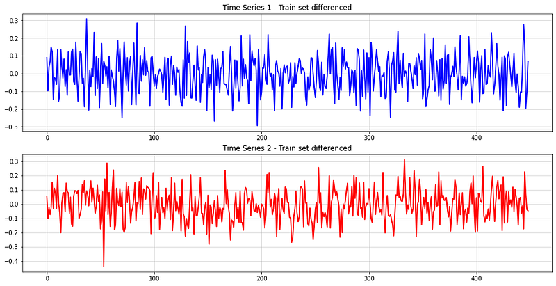
An Augmented-Dickey Fuller test from statsmodels shows significance scores of 0.8171 and 0.8512. This underlines the visible unit-roots in both time-series. Thus, the difference transformation appears to be the logical next step. Let’s do that for the train set to forecast the test set further down the line:

First-differences of the time-series train set. (Image by author)

Next, we can check forecast performance for two VAR(1) models — one trained on the original time-series and one on the transformed one:

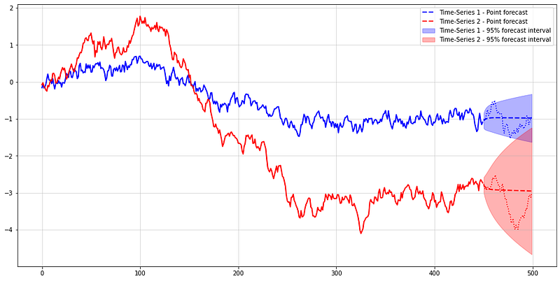
Point- and 95% interval-forecast **without** differencing. (Image by author)

The summed MSE over both time-series forecasts is at 0.3463. Clearly, the model with training data differenced should perform better:

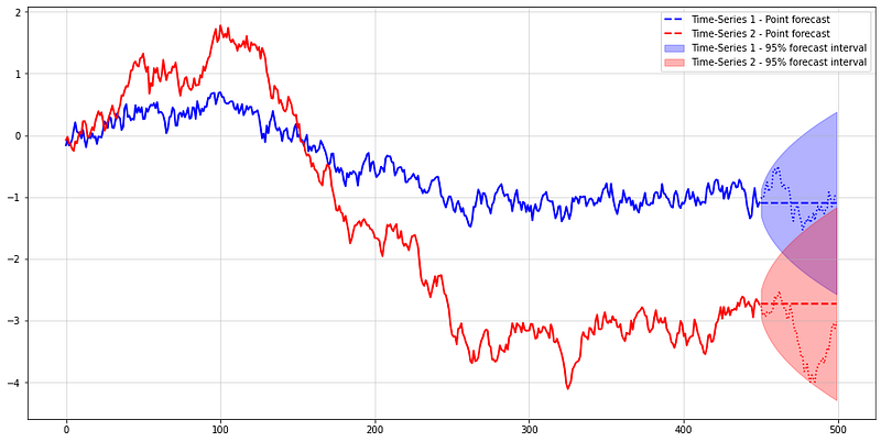
Point- and 95% interval-forecast **with** differencing. (Image by author)

This time, the summed MSE is 0.5105 - approximately 50% higher. Also, the forecast interval for time-series 1 is much larger than without any differencing. Something seems to be off with the popular difference transformation.

Why cointegration matters

Right now, you might — rightfully — argue that the underperformance of the differencing model was due to pure chance. Indeed, we would need much broader experiments to verify our initial claim empirically.

It is, however, possible to actually prove why differencing can be bad for multivariate time-series analysis. To do so, let us take a step back to univariate time-series models and why difference transformations work here.

We will only look at AR(1) and VAR(1) time-series for simplicity. All results can be shown to hold for higher-order AR/VAR, too.

Unit-Root AR(1) time-series — when differencing is likely safe

Mathematically, an AR(1) time-series looks as follows:

In order for differencing to make sense, we need the time-series to have a unit root. This is the case when solution of characteristic polynomial

lies on the unit-circle, i.e.

The only choice for the AR-parameter is therefore

and thus

In order to make this equation stationary, we subtract the lagged variable from both sides:

Clearly, the best possible forecast now is to predict white noise. Keep in mind that we could equally well fit a model on the untransformed variable. However, the differenced time-series directly uncovers the lack of any truly autoregressive component.

On the one hand, differencing is clearly a good choice in univariate time-series with unit-roots. Things are not as simple for multivariate time-series, though.

Multivariate time-series with cointegration

Consider now a VAR(1) time where we replace the scalars in the AR(1) model with vectors (bold, lower-case) and vectors (upper case):

A unit-root in a VAR(1) time-series imply, similarly to the AR(1) case, that

In the trivial case, the autoregression parameter is the identity matrix. This implies that the marginals in our VAR(1) time-series are all independent and unit-root. If we exclude this case and proceed as for AR(1), we get

The last line is also called an Vector Error Correcting Representation of a VAR time-series. If you scroll back to our simulation, this is the exact formula that was used to generate the time-series.

By making Atilde rank-deficient, the time-series becomes cointegrated, as explained by Lütkepohl. There exists another, broader definition of cointegration but we won’t cover that today.

Clearly, a cointegrated VAR(1) time-series differs from the univariate AR(1) case. Even after differencing, the transformed values depend on the past of the original time-series. We would therefore lose important information if we don’t account for the original time-series anymore.

If you are working with multivariate data, you should therefore not just blindly apply differencing.

How to deal with cointegration

The above result begs the question of what we should do to handle cointegration. Typically, time-series analysis is concerned either with forecasting or inference. Therefore, two different approaches come to mind:

Cross-validation and backtesting — the pragmatic, ‘data sciency’ approach. If our goal is primarily to build the most accurate forecast, we don’t necessarily need to detect cointegration at all. As long as the resulting model is performant and reliable, nearly anything goes.

As usually, the ‘best’ model can be selected based on cross-validation and out-of-sample performance tests. The primary implication from cointegration is then to apply differencing with some care.

On the other hand, the above result also suggests that adding the original time-series as a feature might be a good idea in general.

Statistical tests — the classical statistics way. Obviously, cointegration is nothing new to econometricians and statisticians. If you are interested in learning about the generating process itself, this approach is likely mo r e expedient.

Luckily, the work of James MacKinnon provides extensive insights into tests for cointegration. Other popular cointegration tests have been developed by Engle and Granger and Søren Johansen.

In Python, you can find the MacKinnon test in the statsmodels library. For the above time-series, the test yields a p-value of almost zero.

Conclusion

Hopefully, this article was an eye-opener to you to not just difference every time-series straight ahead. You should be aware by now that cointegration is a peculiarity of multivariate time-series that needs to be treated with care.

Keep in mind that standard cointegration is concerned with linear time-series only. Once non-linear dynamics are present, things could become even more messy and differencing might be even less suitable.

Indeed, there exists some recent research on non-linear cointegration. You might want to take a look at it for further details.

References

[1] Engle, Robert F.; Granger, Clive WJ. Co-integration and error correction: representation, estimation, and testing. Econometrica: journal of the Econometric Society, 1987, p. 251–276.

[2] Hamilton, James Douglas. Time series analysis. Princeton university press, 2020.

[3] Lütkepohl, Helmut. New introduction to multiple time series analysis. Springer Science & Business Media, 2005.

Originally published at https://www.sarem-seitz.com on August 25, 2022.