Clustering: concepts, algorithms and applications

… and some experimentation with feature selection and normalization

Let’s do this experiment— take a look at the following figures and see if you can identify which figure has clustered data, A or B?

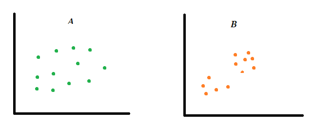
Clustering as a concept is not difficult to understand and I’m not sure if you need to learn anything beyond what you already know. If you answered B, no one else needs to explain to you what clustering is.

In machine learning terminology, clustering is used as an unsupervised algorithm by which observations (data) are grouped in a way that similar observations are closer to each other. It is an “unsupervised” algorithm because unlike supervised algorithms you do not have to train it with labeled data. Instead, you put your data into a “clustering machine” along with some instructions (e.g. # of features & # of clusters), and the machine will figure out the rest and make clusters based on underlying patterns and properties in the data.

So if clustering is such a simple concept then what exactly do we need to learn about them? Quite a few things actually:

• what does clustering mean in practical terms?
• how is this concept used in real-world problem-solving?
• how to quantitatively measure clusters in a large and multi-dimensional dataset?

Let’s crack these questions separately, then we’ll dive into some technical details.

Why clustering? Some use cases

Let’s clear up a few things first. In figure B above the observations are clustered. But in what respect? The answer is — they are clustered in a two-dimensional space with respect to two variables represented by X and Y coordinates.

But that’s just one way to see clusters. Objects can be clustered in a million different ways such as by age, height, location, price, gender — you name it.

Why at Macy’s women’s clothes are all in one place, men’s clothes in a different corner and furniture are probably on an entirely different floor? Why do they organize products in a way that similar things are together and different things are separated? We don’t need data science to understand that. But there are numerous instances where we do need data science to understand how things are clustered and how things to cluster. Here are a few examples:

• In exploratory data analysis (EDA) clustering plays a fundamental role in developing initial intuition about features and patterns in data.
• In statistical analysis, clustering is frequently used to identify the (dis)similarities variables in different samples.
• Insurance industries use clustering for anomaly detection and potentially catch fraudulent transactions.
• Clustering is widely used in customer segmentation — e.g. for developing marketing strategies targeting different groups of customers.
• In computer vision, image segmentation is used to partition data into disjoint groups using pattern recognition.
• Clustering is an essential tool in biological sciences, especially in genetic and taxonomic classification and understanding evolution of living and extinct organisms.
• Clustering algorithms have wide-ranging other applications such as building recommendation systems, social media network analysis etc.
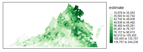
• Spatial clustering helps identify households and communities of similar characteristics to implement appropriate community development and taxation policies.

The clustering algorithms

It’s easy to visualize data in a two-dimensional plane and visually inspect whether they are clustered or not. But what if there are 3 or 4 dimensions; or even 10s of dimensions? What if there are millions or even billions of data points? Algorithms are here to help. Here are a few clustering algorithms frequently used in machine learning:

• K-means
• Hierarchical
• DBSCAN
• Spectral
• Gaussian
• Birch
• Mean shift
• Affinity propagation

Each algorithm above has strengths and weaknesses of its own and is used for specific data and application context.

K-means Clustering is probably the most popular and frequently used one. The algorithm starts with an imaginary data point called “centroid” around which each cluster is partitioned. K-means is easy to implement and interpret. But one key disadvantage is its sensitivity to outliers.

Hierarchical clustering is more informative than K-Means but it suffers from a similar weakness of being sensitive to extreme values. Additionally, implementing this algorithm can be time-consuming for large datasets.

DBSCAN is robust in the presence of outliers but has its own disadvantage — high sensitivity to model parameters (ε and minPts).

I wrote more about these algorithms and their properties in a previous article if you’d like to check out.

Implementation

In this section we will do a rapid implementation of K-Means clustering using sklearn package in a step-by-step approach. In the next section, we will discuss how this simple implementation can be adapted in different situations using different model setups.

Let's first import some libraries.

# importing libraries
import pandas as pd
import numpy as np
import matplotlib.pyplot as plt
import seaborn as sns
from sklearn import preprocessing
from sklearn.cluster import KMeans

Next step is to import data. I am using the famous (and over-used!) Iris dataset for this demonstration. The data is available online and can be imported easily using the code below.

One thing that needs to be made clear here is that the Iris dataset is a “cleaned” dataset — no feature engineering required, no missing values or no filtering required. I’m using it solely to focus on the algorithm, but of course we know that in real-world it takes quite a bit of work to clean them up.

# importing **cleaned** data
df = pd.read_csv("https://raw.githubusercontent.com/uiuc-cse/data-fa14/gh-pages/data/iris.csv")

df.head()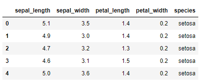

Next up feature selection. In the table above, the dataset contains 5 columns — 4 of which are numeric and one string values. Out of 5, we are going to choose just 2 features in this round (later we’ll see how it works in multiple features space). In a two-dimensional scatterplot this is how it looks like.

# scatterplot
plt.scatter(df["petal_length"], df["petal_width"])
plt.xlabel("Petal length")
plt.ylabel("Petal width")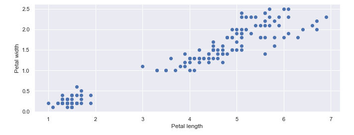

You’ll immediately recognize a cluster is distinguishable in the left lower corner of the plot. But what about the rest of the data points? It’s not that easy to identify whether they are just one cluster or if they could be broken into two or more clusters based on any other underlying features. That’s what an algorithm is good at and we’ll use an example towards the end.

Since we are doing a two-feature cluster analysis let’s select those features below. Normalizing data is also an essential part of input preparation (we’ll talk about normalization later again).

# feature selection
df = df[["petal_length", "petal_width"]]

# normalizing inputs
X = preprocessing.scale(df)

With that minimum data preparation, all that remains is instantiating the K-means algorithm from sklearnand fit the model with input data X. The only parameter we are using is n_clusters to specify the number of clusters we want.

# instantiate model
model = KMeans(n_clusters = 3)

# fit predict
y_model = model.fit_predict(X)

So we have fitted the model, now it’s time to visualize them in a scatterplot.

# visualize clusters
plt.scatter(X[:,0], X[:,1], c=model.labels_, cmap='viridis')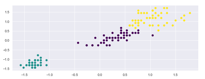

In a visual inspection do the clusters make sense? Pretty good, right? We can now count how many observations fall under each cluster.

# value counts in each cluster
pd.value_counts(y_model)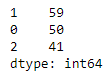

Let’s keep the scatterplot and counts of data in the back of our mind, we’ll need them to compare performance of alternative modeling options. Let’s call this model the “baseline” model.

Technical considerations

In the above, we implemented a model with a set of pre-determined inputs. The purpose of this section is to go beyond the baseline and see how differently we could set up the model and how that impacts clustering. We will do three different experiments:

• Features selection
• Normalization
• Algorithm

Feature selection

Like I said before, you could choose any number of features for creating clusters and in the baseline model we used just two. But what if we select three features instead and how does that impacts the clusters?

Let’s re-run the model with new features.

# feature selection
df = df[["petal_length", "petal_width", "sepal_length"]]

# normalizing inputs
X = preprocessing.scale(df)

# instantiate model
model = KMeans(n_clusters = 3)

# fit predict
y_model = model.fit_predict(X)

print("Value Counts")
print(pd.value_counts(y_model))

# visualize clusters
plt.scatter(X[:,0], X[:,1], c=model.labels_, cmap='viridis')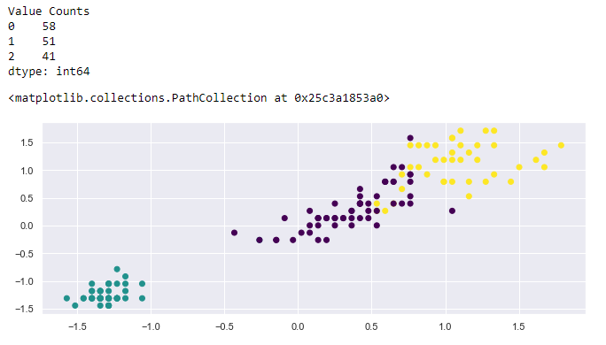

If you compare this new model with the baseline you will see that we still have 3 clusters and the cluster at the bottom corner remains the same. The rest of the clusters have quite a few overlapping data points. This is because we are using a two-dimensional plane to represent 3-dimensional outputs. If we could create a 3D scatterplot the clusters probably wouldn’t be overlapping.

Normalization

Normalization requires a long discussion, but to make a long story really short, the purpose of normalization is to scale data within the same range, let’s say -2 to +2. The benefit of doing so is that it condenses highly scattered/dispersed data so that makes it easy to find clusters.

Let’s re-run with the new setup.

# feature selection
df = df[["petal_length", "petal_width"]]

# inputs (NOT normalized)
X = df.values

# instantiate model
model = KMeans(n_clusters = 3)

# fit predict
y_model = model.fit_predict(X)

# visualizing clusters
plt.scatter(X[:,0], X[:,1], c=model.labels_, cmap='viridis')

# counts per cluster
print("Value Counts")
print(pd.value_counts(y_model))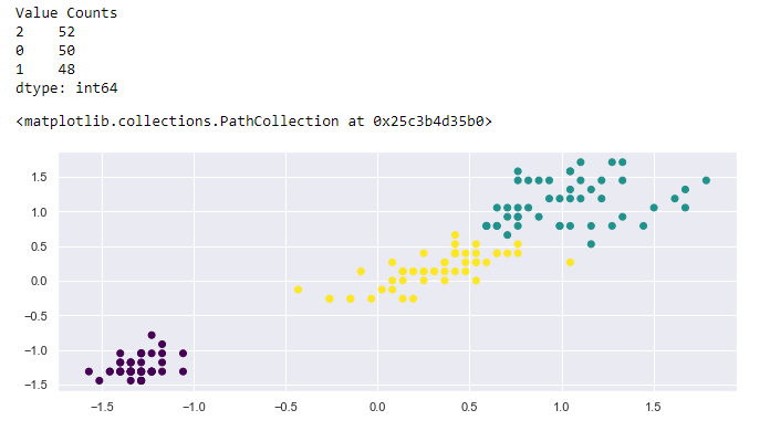

Homework: Can you now compare the 3-feature outputs with the 2-feature outputs in the baseline? You can visually inspect in also see the value counts.

Algorithm

We talked about quite a few algorithms that can be used for clustering and each has advantages and disadvantages. There is no algorithm that is better or worse in *absolute* sense, it just depends on the underlying data structure and the feature space. In real-world you will need to experiment with several algorithms and see which one does a good job.

Let’s set up the model with a different algorithm, this time using hierarchical clustering, keeping others the same, and compare the results with the baseline model.

# import model
from sklearn.cluster import AgglomerativeClustering

# feature selection
df = df[["petal_length", "petal_width"]]

# normalizing inputs
X = preprocessing.scale(df)

# instantiate model
model = AgglomerativeClustering(n_clusters=3, affinity='euclidean', linkage='ward')

# fit/predict model
y_model= model.fit_predict(X)

# ploting clusters
plt.scatter(X[:,0], X[:,1], c=model.labels_, cmap='viridis')

# counts per cluster
print("Value Counts")
print(pd.value_counts(y_model))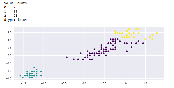

Determine the number of clusters

This is a bonus part. So we kind of arbitrarily specified 3 clusters in the baseline model and subsequent experiments. It was easy to determine from visual inspection because it’s a tiny dataset. But actually, there is a data-driven approach to make that determination — called the Elbow method. The code snippet below may look a bit complex than it should be but don’t put an extra effort to understand it if you don’t want to.

# determine number of clusters using "elbow method"
k_range = range(1,10)
sse = [] # we want to minimize SSE
for k in k_range:
    m = KMeans(n_clusters=k, random_state=0)
    m.fit(X)
    sse.append(m.inertia_)
    
plt.xlabel("K")
plt.ylabel("Sum of squared errors")
plt.plot(k_range, sse, marker='x')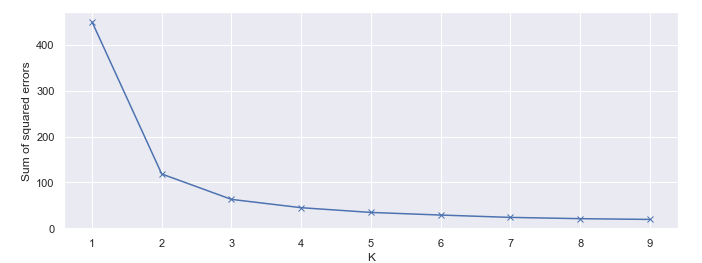

What the Elbow method does is help us heuristically decide the number of clusters based on a cutoff point (k = 3), beyond which adding more clusters does not significantly reduce the sum of squared errors. That’s the point that looks like a human elbow.

Summary

I’ve covered several different themes in this article, it’s time to summarize them:

• clustering is simple as a concept but needs help with machines to implement for a large and/or multi-dimensional dataset
• use cases are wide-ranging — from descriptive statistics, anomaly detection and recommendation systems design to biology, spatial statistics and urban planning
• several algorithms are in the market but popular ones are — K-means, hierarchical and DBSCAN clustering
• with cleaned data, running and interpreting cluster analysis with sklearn is an easy task
• number of features, normalization and algorithms can make differences in how clustering is done

I hope this was a useful article. If you have comments feel free to write them down below. You can follow me on Medium, Twitter or LinkedIn.