
Fashion AI
Clothes Classification with the DeepFashion Dataset and Fastai
A story of how I started cleaning my wardrobe and ended up training a neural network

The first of January is a perfect day to sort out your winter clothes. That’s what I had in mind when approaching my wardrobe a month ago. The monotonic process of folding sweaters, socks, and scarves is quite meditative by nature and leads to many discoveries. Like the one that I have three pink blouses of the same style. This discovery helped me to realize that I inevitably need to optimize my fashion inventory by increasing the diversity and decreasing the redundancy of the items I own. Naturally, the goal should be to model the content of my wardrobe as a graph that will incorporate clothing items, their type (sweater, pants, etc.), attributes (fabric, style, color, etc.), and relations (whether two items can be combined in one look or not). In this article, I am writing about the approach that I took for creating my dataset, specifically how to recognize the clothes type of a random item.
This article contains the following parts:
- Data
- Model training
- Model evaluation
- How to load a pre-trained model from Fastai to PyTorch
- Summary
Even though I am using Keras for Deep Learning for years, this time I decided to give PyTorch and Fastai a try. The full code used in the article can be found here.
Data
To categorize items in my wardrobe, I need to have a model that is trained to solve that task, and to train such a model I need data. In this project, I used the DeepFasion Dataset which is a large-scale clothes database for Clothing Category and Attribute Prediction, collected by the Multimedia Lab at the Chinese University of Hong Kong.
The classification benchmark was published in 2016. It evaluates the performance of the FashionNet Model in predicting 46 categories and 1000 clothes attributes. For the original paper please refer to DeepFashion: Powering Robust Clothes Recognition and Retrieval with Rich Annotations, CVPR 2016.
The DeepFashion Database contains several datasets. In this project, the Category and Attribute Prediction Benchmark was used. This dataset contains 289,222 diverse clothes images from 46 different categories.
The training labels are stored at train_labels.csv in the following format:
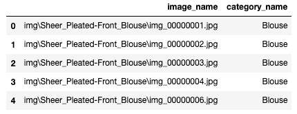
The training data file contains the location of the images and the labels. Labels are stored as a string object, one label per image.
We can load the data from the train_labels.csv to the ImageDataLoaders class using the from_csv method.
I am using a Fastai data augmentation strategy called presizing. It resizes the images to a smaller square shape first. That enables all the following augmentations to happen faster as the square images can be processed on a GPU. Then we can apply augmentation to each data batch. batch_tfms performs all augmentations like rotation and zoom sequentially, with a single interpolation at the end. This augmentation strategy will allow us to achieve a better quality of augmented images and gain some speed due to the processing on GPU.
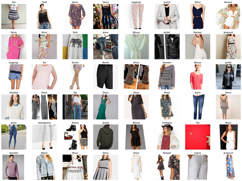
Let’s look at some images in our dataset.
We can also check how the augmented images look by passing unique=True to the show_batch method above.
As we can see, images preserved their quality after the augmentation.
Model Training
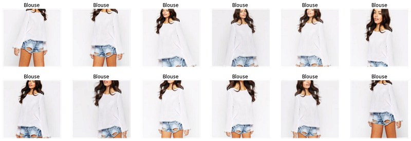
In this project, I am using the pre-trained ResNet34 model. I experimented with deeper architectures, but they didn't lead to a significant improvement. The main challenge of the DeepFashion dataset is the quality of labels. For example, the image above shows two items: blouse and shorts, but it has only a “blouse” label. This way the model will inevitably suffer from noise.
To make transfer learning work, we need to replace the last layer of the network with a new linear layer containing the same number of activations as the number of classes in our dataset. In our case we have 46 clothes categories, meaning that we have 46 activations in our new layer. The newly added layer initializes weights at random. Therefore our model will have random output before it is trained, which doesn’t mean that the model is entirely random. All the other layers that were not changed will preserve the same weights as the original model and will be good at recognizing general visual concepts such as basic geometric forms, gradients, etc. Therefore when we are training our model to be able to recognize clothes types, we freeze the entire network except for the last layer. That will allow us to optimize the weights of the last layer without changing the weights of the deeper layers.
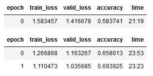
When we call learn.fine_tune(), we freeze the entire network and train the randomly initialized weights of the newly created layer for one epoch. Then we unfreeze the network and train all the layers together for the number of epochs we specified (in our case two). That is why we see one extra epoch in the output.
Early Evaluation
Early evaluation allows us to check the learning progress on the earlier stages and catch mistakes in our approaches before we spent a lot of time training the model. There are multiple ways to look at the results produced by training a neural network. To get a quick impression we can look at the most frequently confused classes:
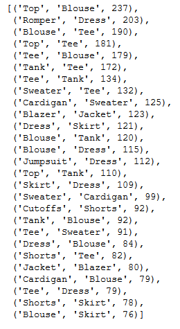
As we can see the network most often confuses ‘Top’ with ‘Blouse’, ‘Romper’ with ‘Dress’, and ‘Tee’ with ‘Blouse’. Even a human could make such mistakes. This way we can early evaluate whether our network learns the right pattern.
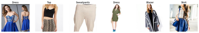
Another way to look at the errors is to plot top losses.
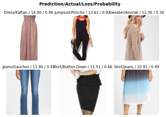
As mentioned above, the original labels are noisy. Our model correctly classified a Jumpsuit, two Skirts, and a Dress, while in the original dataset these items have the wrong labels.
Learning Rate Finder
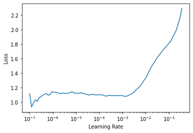
Now let’s go through the data in the DataLoader and gradually increase the learning rate with each mini-batch to observe how the value of loss changes with the change of learning rate. Our goal is to find the most efficient learning rate that will allow the network to converge faster. The learning rate has an optimal value at the point of the steepest slope of the loss curve, as it means that loss decreases faster. The points of extremums (min and max) and flat parts of the curve correspond to the learning rates that do not allow the network to learn, as the loss at these points does not improve.
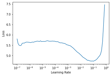
In our case, the steepest point of the loss curve is at the learning rate equal to 0.005. This learning rate we will use for further training.
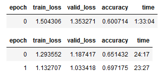
After training the model for 3 epochs, we got an Accuracy of 0.697 which is an improvement over 0.694, that we had with the default learning rate.
Discriminative Learning Rates
After training all layers of the network we need to review the learning rates again, as after a few batches of training the speed with which the network learns slows down and we are risking to overshoot the minimum of the loss function with high learning rates. Therefore the learning rate requires to be decreased.
When we plot the Loss Curve after three epochs of training, we can see that it looks different, as the weights of the network are not random anymore.
We do not observe this sharp decrease associated with the point where the weights were updated from random to ones which decreases the loss. The shape of the curve looks flatter. For future training, we will take a range of weights from the point of decrease till the point where the loss starts growing again.
As was mentioned previously, the layers transferred from the pre-trained model are already good at recognizing fundamental visual concepts and do not require much training. However, deeper layers that are responsible for recognizing complex shapes specific to our project will benefit from higher learning rates. Therefore we need to use smaller learning rates for the first layers and bigger learning rates for the last layers to allow them to fine-tune more quickly.
We definitely can see that our network makes progress in learning. However, it is hard to say whether we need to continue the training, or stop to not overfit the model. Plotting the training and validation loss can help us to evaluate whether we need to continue.
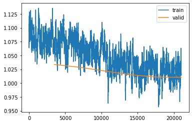
We can see that the validation loss doesn't improve that much anymore, even though the training loss is still improving. If we continue training, we will increase the gap between the training and validation loss which will mean that we overfitted our model. Therefore we better stop the training now and go to the next step, evaluation.
Model Evaluation
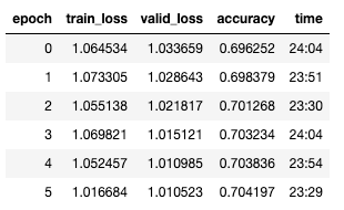
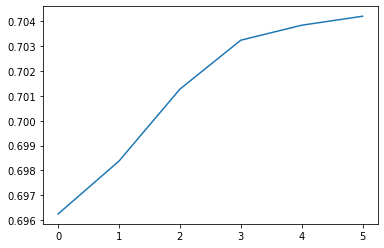
In the previous step, we were able to achieve 70,4% Top-1 Accuracy on the validation dataset. If we plot the validation accuracy, we can see how it was improving with each epoch.
Evaluation on the Training Dataset
First, we will look at the predictions on the training dataset to estimate if we still have a high bias.
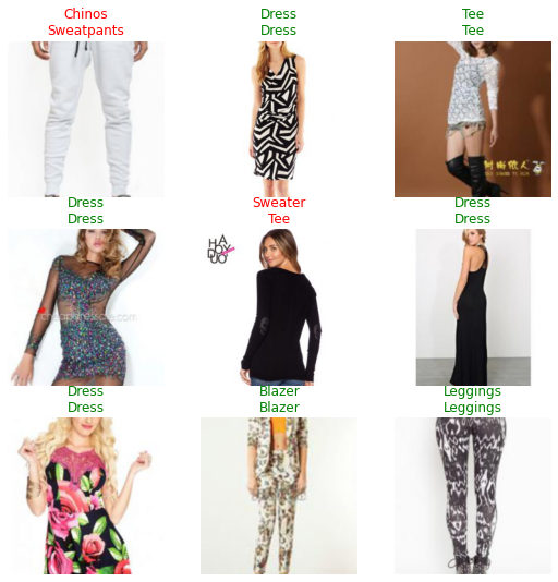
The predictions on the training dataset look good. Our model captures the main concepts. Further improvements can be achieved by improving the labels and cleaning the data.
Evaluation on the Test Dataset
Now let’s load the test data and check how the model performs on it.
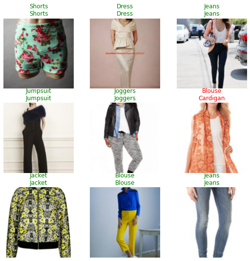
The model Top-1 Test Accuracy is 70,4%. It misclassifies a few objects but still very close to the result we got on the validation set.
The authors of the original paper DeepFashion: Powering Robust Clothes Recognition and Retrieval with Rich Annotations, CVPR 2016 used Top-3 and Top-5 accuracy for the evaluation.
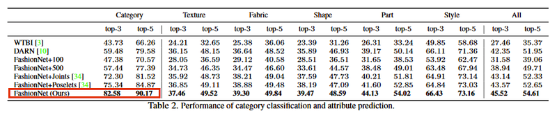
To make our results comparable, I will use the same metrics.
The Top-3 Accuracy of our model is 88.6%, which is 6% higher than the benchmark accuracy and the Top-5 Accuracy of our model is 94.1%, which is 4% higher than the benchmark accuracy. This should not come as a surprise as the authors of the original paper used VGG16 architecture as a backbone, which is a less powerful model.
Evaluation on a User Specified Dataset
Finally, we will check how the model works with my images. I took 98 pictures of my own clothes with a smartphone camera. Let’s load the images and check whether the model can classify them correctly.
The Top-1 Accuracy of the model on the user-specified data is 62.4% which is lower than on the DeepFashion Dataset. However, it is still good for a 46 class classification model.
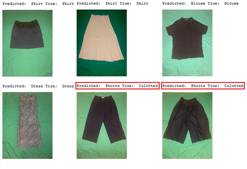
The images in the user dataset are quite different from those on which the model was originally trained. For example, user images only show a clothes item, while the images in the DeepFashion dataset show a human wearing an item which makes it easier to scale the clothes. Almost all the pants in the user dataset were classified as shorts as it is hard for a model to estimate its lengths relative to the human body. Nevertheless, the model learned the main concepts and could be used in a variety of fashion contexts.
How to load a pre-trained model from Fastai to PyTorch
After training the model, we might want to run it on an inference machine without Fastai installation. For that we first need to save the model and its vocabulary:
torch.save saves the weights of the pre-trained model. It uses Python’s pickle utility for serialization. To run the model in PyTorch, we need to load the weights and redefine the model:
Note that this time we need to resize and normalize images before running the prediction. The Fastai library stores information about the transformations to be applied in the learner, but when we run the model outside of Fastai, we need to transform the images first.
After that we can run predictions using the class we defined:
Summary
In this tutorial, I showed how to train a ResNet34 model for clothes type recognition using the Fastai library and DeepFashion Dataset. We have seen that we can train a model that will outperform the current baseline by 6% for Top-3 Accuracy and by 4% for Top-5 Accuracy. We run an evaluation on my own images and observed that the model classifies items correctly except for scale sensitive items (shorts or pants problem). The model performance can benefit from improving the quality of the training labels and increasing the diversity of the images.
This is just the very beginning of the fashion project that I have in mind. The article about attribute, pattern, and fabric recognition will come next. Stay tuned!
Thanks for reading this article! Leave a comment below if you have any questions or reach me on LinkedIn.


