Hands-on Tutorials

Classifying Images of Alcoholic Beverages with fast.ai v2

Using fast.ai v2 and Google Colab to serve an intoxicating mix of data and dram

Motivation

Having starting immersing myself in the updated fast.ai v2 deep learning course, I felt it would be ideal to apply and document what I have learnt so far. In this article, I will be sharing about how I trained a deep learning (CNN) classifier to distinguish the different types of popular alcoholic beverages.

An important highlight of this walkthrough is that it details the latest instructions on how to utilize the updated Microsoft Azure Bing Search V7 API, since key changes were implemented as of 30 Oct 2020.

Links

• GitHub Repo
• Jupyter Notebook (Full Version)
• Jupyter Notebook (Clean version)

Contents

Section 1 — Setup

Section 2 — Downloading Image Data

Section 3 — Preparing Image Datasets

Section 4 — Training the Model

Section 5 — Cleaning the Data

Section 6 — Using Image Classifier for Inference

Section 7 — Deployment as Web App

Section 1 — Setup

First things first, I would highly recommend running this notebook on Google Colab. To find out more about Google Colab setup, please visit this link.

Once this notebook is open on Google Colab, do switch on the GPU accelerator for the notebook by heading to the top menu and clicking Runtime > Change runtime type > Select GPU for Hardware Accelerator.

Next, mount your Google Drive on your Google Colab runtime. A link will appear for you to click and retrieve your authorization code. After granting permission to Google Drive File Stream, copy the code provided, paste it in the field under ‘Enter your Authorization Code’, and press Enter.

from google.colab import drive
drive.mount('/content/drive/')

The next step is to install the fast.ai dependencies. I found this combination of dependency versions to be working smoothly on Google Colab.

!pip install fastai==2.0.19
!pip install fastai2==0.0.30
!pip install fastcore==1.3.1
!pip install -Uqq fastbook

import fastbook
from fastbook import *
fastbook.setup_book()
from fastai.vision.widgets import *

import warnings
warnings.filterwarnings("ignore")

import requests
import matplotlib.pyplot as plt
import PIL.Image
from io import BytesIO
import os

from IPython.display import Image
from IPython.core.display import HTML

We then create a path to store the images that we are about to download. Note that the resultant directory path will be /content/images.

try:
  os.mkdir('images')
except:
  pass

After that, we need to retrieve the API key for Azure Bing Search V7, since we will be using it to pull image datasets from Bing. To find out more about setting up the Bing Search API key in the Microsoft Azure Portal, please have a look at the README file in my GitHub repo, as well as the Microsoft Azure Bing Search API quickstart guide.

subscription_key = "XXX" #Replace XXX with your own API key
search_url = "https://api.bing.microsoft.com/v7.0/images/search"
headers = {"Ocp-Apim-Subscription-Key" : subscription_key}

Once the key has been entered into the subscription_key variable, we can retrieve a set of image URLs related to the keyword of your choice. For example, to find a set of images for whisky, we run the following code:

search_term = "whisky"

#Add in count parameter so that max number of images (150) is  #retrieved upon each API call. Otherwise, default is 35.

params  = {"q": search_term, "license": "public", "imageType": "photo", "count":"150"}

response = requests.get(search_url, headers=headers, params=params)
response.raise_for_status()

# Return json file
search_results = response.json()

# Create a set of thumbnails for visualization
thumbnail_urls = [img["thumbnailUrl"] for img in search_results["value"][:16]]

We can create a 4 x 4 grid plot of thumbnails to visualize the images retrieved, allowing us to verify that the images do represent our keyword whisky. From what is displayed, it does look very much like good ol’ whisky to me.

f, axes = plt.subplots(4, 4)
for i in range(4):
    for j in range(4):
        image_data = requests.get(thumbnail_urls[i+4*j])
        image_data.raise_for_status()
        image = Image.open(BytesIO(image_data.content))        
        axes[i][j].imshow(image)
        axes[i][j].axis("off")
plt.show()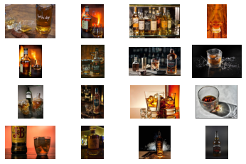

The next step is to collate the list of image URLs from the search results JSON file. The key that is associated with the image URL is contentUrl.

img_urls = [img['contentUrl'] for img in search_results["value"]]
len(img_urls)

The len function should return us a list of 150 image URLs related to the keyword whisky. We then download and display a single image from a URL into the destination file named whisky_test.jpg inside our images folder.

dest = 'images/whisky_test.jpg'
download_url(img_urls[1], dest)

img = Image.open(dest)
img.to_thumb(224,224)

We got ourselves a whisky image above, showing that the chunks of code above worked perfectly. We are now ready for the main action.

Section 2 — Downloading Image Data

Update: As the image download method is dynamic, please refer to the fast.ai Images section to find out what is the latest approach for image downloads

It would be interesting to distinguish the images of common alcohol types, namely whisky, wine and beer. To do that, we first define the three alcohol types in a list, and create a Path to store the images we are going to download shortly.

alcohol_types = ['whisky','wine','beer']
path = Path('alcohol')

For each of the three alcohol types, we create a subpath to store the images, and we proceed to download the images from the image URLs collated.

if not path.exists():
    path.mkdir()
    for alc_type in alcohol_types:
        dest = (path/alc_type)
        dest.mkdir(exist_ok=True)
        
        search_term = alc_type
        params  = {"q":search_term, "license":"public",   
                   "imageType":"photo", "count":"150"}
        response = requests.get(search_url, headers=headers, 
                   params=params)
        response.raise_for_status()
        search_results = response.json()
        img_urls = [img['contentUrl'] for img in   
                    search_results["value"]]
        
        # Downloading images from the list of image URLs
        download_images(dest, urls=img_urls)

We should now have the images downloaded within the respective folders with the label of the alcohol type. To confirm this, we can utilize the get_image_files function.

img_files = get_image_files(path)
img_files

(#445) [Path('alcohol/beer/00000069.jpeg'),Path('alcohol/beer/00000007.jpg'),Path('alcohol/beer/00000092.jpg'),Path('alcohol/beer/00000054.jpg'),Path('alcohol/beer/00000082.jpg'),Path('alcohol/beer/00000071.jpg'),Path('alcohol/beer/00000045.jpg'),Path('alcohol/beer/00000134.jpg'),Path('alcohol/beer/00000061.jpg'),Path('alcohol/beer/00000138.jpg')...]

Another method to verify the downloads is to click on the Files icon on the left navigation bar of the Google Colab screen, and navigate to content>alcohol to see the respective folders.

After that, we need to check whether the files we downloaded are corrupt or not. Fortunately, fastai provides a convenient way to do just that, via theverify_images function.

failed = verify_images(img_files)
failed

We can then proceed to remove these corrupt files (if any) from our dataset, using the map and unlink methods.

failed.map(Path.unlink)

Section 3 — Preparing Image Datasets

fastai has a flexible system called the data block API. With this API, we can fully customize the creation of the DataLoaders object. DataLoaders can store whatever DataLoader objects we place in it, and it is used to generate training and validation sets subsequently.

In my interpretation, DataLoaders is essentially an object that stores information about the data we will run our model on. The DataBlock is basically a template function for creating DataLoaders.

alcohols = DataBlock(
    blocks=(ImageBlock, CategoryBlock), 
    get_items=get_image_files, 
    splitter=RandomSplitter(valid_pct=0.2, seed=1),
    get_y=parent_label,
    item_tfms=Resize(128))

Let’s go through the above code part by part:

blocks=(ImageBlock, CategoryBlock)

This blocks tuple indicates the data types for our independent and dependent variables respectively. Since our aim here is to classify images, our independent variable is images (ImageBlock) while our dependent variable is categories/labels (CategoryBlock)

get_items=get_image_files

The get_items argument specifies the function to be used in order to extract the file paths of the images in our dataset. Recall we earlier used the fastai built-in get_image_files to get the file paths into the variable img_files. This get_image_files function takes a path (which we will specify later), and returns a list of all of the images in that path.

splitter=RandomSplitter(valid_pct=0.2, seed=1)

The splitter method will split the dataset into training and validation sets. We specify RandomSplitter to ensure that it is split randomly, and the valid_pct argument within it is there to indicate what percentage of the dataset is to be allocated as a validation set. The random seed can also be set within the RandomSplitter for reproducibility of results.

get_y=parent_label

parent_label is a function provided by fastai to get the name of the folder the image files are located in. Since we have placed our images in folders with the respective alcohol type name, this parent_label will be returning the folder names of whisky, wine and beer.

item_tfms=Resize(128)

We normally use resize images into a square as it is easier to do so, since original images can come in different height/width and aspect ratio. To do this, we perform a transformation on each item (item_tfms) by resizing it into squares of 128x128 pixels.

Now that all the details and arguments have been provided, we can then proceed to initiate the DataLoaders with the following single line of code. Notice that the argument for dataloaders is the path where our images are stored i.e. alcohol folder path.

dls = alcohols.dataloaders(path)

Let’s have a brief look at the images by showing a subset batch of 10 images inside our validation set

Note: The following display of image thumbnails is a good way to validate whether the data download was performed correctly. Previously when I ran this code, I realise that I did not update the search_term accordingly, resulting in all images being that of whisky. If done correctly, the following batch should show a myriad of the images from different categories.

dls.valid.show_batch(max_n=12, nrows=2)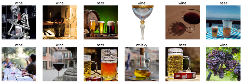

Demonstrating How Data Augmentation Works

Before proceeding further, it is important to talk about the concept of data augmentation. In order to enrich our training dataset, we can create random variations of our input data, such that they appear different, but do not actually change the original meaning and representation of the data.

A common way to do this includes RandomResizedCrop, which grabs a random subset of the original image. We use unique=True to have the same image repeated with different versions of theRandomResizedCrop transformation.

What happens is that on each epoch (which is one complete pass through all of our images in the dataset), we randomly select a different part of each image. This means that our model can learn to recognize different features in our images. It also reflects how images work in the real world, since different photos of the same item may be framed in slightly different ways. The benefit of using item transformation is that it in turn helps to prevent overfitting.

The min_scale parameter specified determines how much of the image to select at minimum each time. With all the above decided, we can create a new DataBlock object using the .new method, and running it to give us a new DataLoaders object named dls.

alcohols = alcohols.new(item_tfms=RandomResizedCrop(128, min_scale=0.3))
dls = alcohols.dataloaders(path)
dls.train.show_batch(max_n=8, nrows=2, unique=True)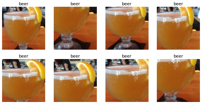

Following the item transformation (item_tfms), we run batch transformation (batch_tfms) where we apply a standard set of data augmentation transformations (aug_transforms()) on the batch of the individual items.

The difference between item_tfms and batch_tfms is that item_tfms performs the transformation on every individual item (e.g. image), whereas batch_tfms runs transformation on an entire batch of items.

The following code illustrates the effects of the augmentation transformation aug_transforms on a single input image. You will be able to observe some form of rotation, perspective warping and contrast changes.

alcohols = alcohols.new(item_tfms=Resize(128), batch_tfms=aug_transforms())
dls = alcohols.dataloaders(path)
dls.train.show_batch(max_n=8, nrows=2, unique=True)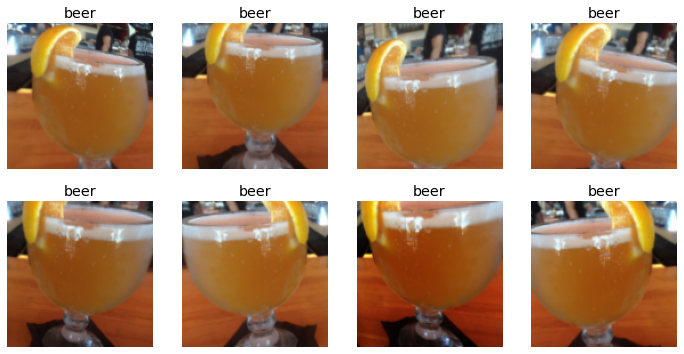

Section 4 — Training the Model

Now that the images are prepared (albeit not cleaned yet), we can start the training to build a simple deep learning model right off the bat. First we prepare the DataLoaders object with the following code. In this iteration, we resize and crop our images at sizes of 224x224 pixel, with min_scale of 0.5.

alcohols = alcohols.new(
    item_tfms=RandomResizedCrop(224, min_scale=0.5),
    batch_tfms=aug_transforms())
dls = alcohols.dataloaders(path)

Convoluted neural network (CNN) is the de facto type of neural network used for image classification, and that is what we will be using. In terms of the architecture, I arbitrarily chose resnet34 (i.e. 34 layers deep) for the cnn_learner fast.ai function. Details of resnet can be found here.

We are using the .fine_tune method instead of .fit because we are leveraging on the pretrained resnet model to perform transfer learning. We specify the number of epochs to be 4 (i.e. argument inside .fine_tune).

learn = cnn_learner(dls, resnet34, metrics=error_rate)
learn.fine_tune(4)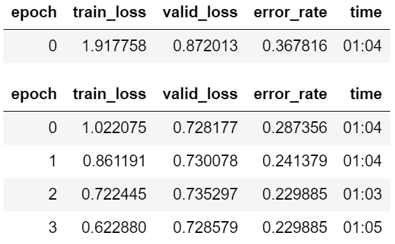

From the above, we can see that after training our CNN learner for a couple of minutes, we obtain an error_rate of 0.229 (i.e. 77.1% accuracy). Not a bad start, given that we have not yet cleaned our dataset.

Using the Confusion Matrix allows for better visualization of the results.

interpretation = ClassificationInterpretation.from_learner(learn)
interpretation.plot_confusion_matrix()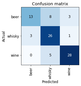

fast.ai also provides a easy method that allows us to find out which are the images where there was the highest loss. The loss is a number that is higher if the model is incorrect (especially if it is also confident of its incorrect answer), or if it is correct, but not confident of its correct answer. These helps us identify the images which the model had trouble with.

interpretation.plot_top_losses(5, nrows=1)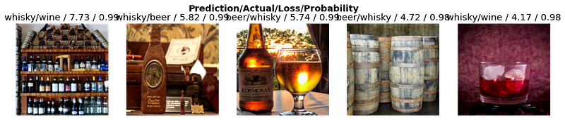

From the above, it appears that some of the problem stems from the fact that several actual labels were labelled incorrectly, instead of the predictions being wrong.

For example, the image in the middle of the row is quite clearly that of a pint of beer (which is exactly what the model predicted). However, the actual label assigned to it was whisky, which is incorrect. This highlights the importance of having correctly labeled data (as much as possible) before training any kind of machine learning model.

Section 5 — Cleaning the Data

Notice that we ran the model before cleaning the data. In fact, doing so makes the data cleaning even easier subsequently. As shown above, the plot_top_losses can already indicate which are the images that the model has most trouble with.

The data cleaning process is made easy with the in-built fast.ai ImageClassifierCleaner Graphical User Interface (GUI) widget.

cleaner = ImageClassifierCleaner(learn)
cleaner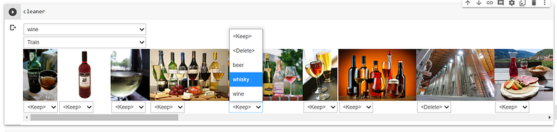

The row of images displayed are the images where the loss was highest, and this GUI gives you an opportunity to review and amend them.

The cleaning is done by selecting a dropdown option for each of the images above, and then running the ‘cleaning’ code iteratively. I took some time to figure this out since the online explanations were unclear, so here are some further details:

• Step 1: After a row of images is loaded in the cleaner output cell (e.g. Training set for Wine category), select a dropdown option for the images that you wish to edit, based on your own judgement. The options consist of deleting the image from the dataset, or moving the image into a new category. If no changes are needed, there is no need to select any option since the default option is .
• Step 2: Once you are done updating the options for the row of images on display, run the following ‘cleaning’ code to execute the changes.

# Delete images marked as delete
for idx in cleaner.delete(): cleaner.fns[idx].unlink()
    
# Update category of image to the newly specified category by moving # it into the appropriate folder
for idx,cat in cleaner.change(): shutil.copyfile(cleaner.fns[idx], path/cat)

cleaner.delete removes the images you have tagged as <Delete>, while cleaner.change shifts the image into the folder with the updated label.

• Step 3: Head back to the cleaner cell with the row of images again, and switch to a new set of images via the dropdown menu e.g. Validation set of Beer category, or Training Set of Whisky category
• Step 4: After the new row of images is loaded, select the relevant dropdown options for each of the images, and then re-run the ‘cleaning’ code
• Step 5: Repeat steps 3 and 4 iteratively for each dataset until all the datasets have been reviewed at least once.

Retraining the model after data cleaning

dls = alcohols.dataloaders(path)
learn = cnn_learner(dls, resnet34, metrics=error_rate)
learn.fine_tune(4)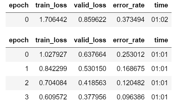

With just a little bit of data cleaning (mostly by removing irrelevant images with the .unlink method), we see a huge improvement in the error_rate (decreased from 0.229 to 0.096). This means that the accuracy has increased from the earlier 77.1% (before data cleaning) to the current 90.4%.

interpretation = ClassificationInterpretation.from_learner(learn)
interpretation.plot_confusion_matrix()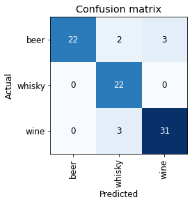

From the confusion matrix above, we can clearly see that the model has become better at distinguishing between the three types of alcohol beverages.

After the training is complete, we want to export the model so that the architecture, trained parameters and DataLoaders setup is saved. All these will be saved into a pickle (.pkl) file.

learn.export()

path = Path()
path.ls(file_exts='.pkl')

(#1) [Path('export.pkl')]

Section 6 — Using Image Classifier for Inference

After loading the pickle file containing the information of our deep learning image classification model, we can use it to infer (or predict) the label of new images. The model is now loaded into the learner variable learn_inf.

learn_inf = load_learner(path/'export.pkl')

We use a sample image to test our model

# Sample image
ims = ['https://alcohaul.sg/products/i/400/5f7edfe79ae56e6d7b8b49cf_0.jpg']
dest = 'images/test_whisky.jpg'
download_url(ims[0], dest)

im = Image.open(dest)
im.to_thumb(224,224)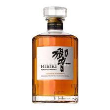

Our sample image is that of a Hibiki Harmony whisky. Let’s see if our model is able to recognize its category.

learn_inf.predict('images/test_whisky.jpg')

('whisky', tensor(1), tensor([4.1783e-04, 9.9951e-01, 7.0310e-05]))

learn_inf.dls.vocab

['beer', 'whisky', 'wine']

Looks like all is good. The model is able to determine with high confidence that the test image represents an image of a whisky (with a probability of 99.95%).

Section 7 — Deployment as Web App

Let’s briefly explore the deployment of the model. We first create a button for users to upload new images which they wish to classify.

We then make use of the PIL.Image.create method to retrieve the uploaded image and store it in the img variable

btn_upload = widgets.FileUpload()
btn_upload

# Retrieving the uploaded image
img = PIL.Image.create(btn_upload.data[-1])

We then setup an Output widget to display the uploaded image.

out_pl = widgets.Output()
out_pl.clear_output()
with out_pl: display(img.to_thumb(224,224))
out_pl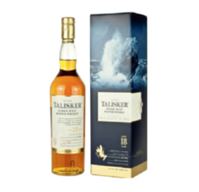

The user has uploaded a Talisker 18 whisky image. It is now time to once again test the classification ability of the model we have built.

pred,pred_idx,probs = learn_inf.predict(img)

lbl_pred = widgets.Label()
lbl_pred.value = f'Prediction: {pred}; Probability: {probs[pred_idx]:.04f}'
lbl_pred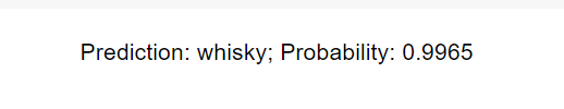

From the above, we can see that our model is indeed predicting the image to be that of a whisky (with 99.65% probability). We can now continue building our web app by including a Run button for users to click and initiate the classification process.

btn_run = widgets.Button(description='Classify Image')
btn_run

Button(description='Classify Image', style=ButtonStyle())

We then setup a callback such that the button above can carry out a specific function upon click. What we want is that whenever the user clicks ‘Classify Image’ for the image he/she uploaded, the classification model will run and then generate a classification prediction.

def on_click_classify(change):
    img = PIL.Image.create(btn_upload.data[-1])
    out_pl.clear_output()
    with out_pl: display(img.to_thumb(128,128))
    pred,pred_idx,probs = learn_inf.predict(img)
    lbl_pred.value = f'Prediction: {pred}; Probability: {probs[pred_idx]:.04f}'

btn_run.on_click(on_click_classify)

And now, putting it all together inside a VBox so that the widgets are arranged nicely in a vertical web app template within our notebook.

VBox([widgets.Label('Select your alcohol!'), 
      btn_upload, btn_run, out_pl, lbl_pred]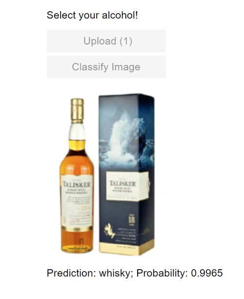

Further Steps

In order to deploy this app outside of this notebook, we can make use of Voila to create a form of real standalone app (built upon Jupyter notebook).

As this aspect is beyond the scope of this notebook, please feel free to explore the details of Voila here.

Conclusion

With that, we have come to the end of this tutorial. We discussed an end-to-end modeling experience, from fast.ai and Google Colab setup, to data ingestion, and all the way to setting up a simple web app for the model we built.

I will continue to post further walkthroughs as I continue my fast.ai learning journey. Meanwhile, time for a drink. Cheers!

Before you go

I welcome you to join me on a data science learning journey! Follow this Medium page and check out my GitHub to stay in the loop of more exciting data science content.