
Causal Inference One-to-one Propensity Score Matching Using R MatchIt Package
How both Python users and R users can use R MatchIt package for causal inference with Propensity Score Matching (PSM)

Propensity Score Matching (PSM) for causal inference using the R MatchIt package is introduced in this tutorial.
Causal inference has well-established packages in R, but not in Python. This tutorial provides an example of using R packages for causal analysis in a Python notebook.
- If you are a Python user, please follow the steps in the tutorial to set up the environment to run the R package MatchIt for propensity score matching. To learn more about how to run R in a Python notebook, please check out my previous tutorial How to Use R with Google Colab Notebook.
- If you are an R user, please ignore the python code and use the R code directly. R code are the ones starting with
%Ror%%R.
In this tutorial you will learn:
- How do the Propensity Score Matching (PSM) algorithms work?
- How to conduct Propensity Score Matching (PSM) using the R package MatchIt?
- How to check the balance of the matched dataset?
- How to calculate causal impact using a t-test or a regression model?
Resources for this post:
- Video tutorial for this post on YouTube
- Python code is at the end of the post. Click here for the Colab notebook.
- More video tutorials on Causal Inference
- More blog posts on Causal Inference
Let’s get started!
Step 0: Propensity Score Matching (PSM) Algorithms for Causal Inference
Propensity Score Matching (PSM) takes a sample in the treatment group and finds a sample with a similar propensity score in the non-treatment group. The goal of matching is to create the treatment and the control groups that are comparable.
The Propensity Score Matching (PSM) process involves the following steps:
- Create a matching dataset based on similarities in the probability of getting the treatment. The probability of getting the treatment is called the propensity score.
- Evaluate the balance of the matched dataset.
- If the matched dataset is balanced, meaning that the test and control dataset has similar confounders, move forward to the next step.
- If the matched dataset is not balanced, go back to the first step, adjust the hyperparameters, and redo the propensity score matching.
- Measure the causal impact. In this tutorial, we will introduce a statistical and a modeling method to measure the impact of the treatment.
Step 1: Install and Import Libraries
In step 1, we will install and import libraries.
Firstly, let’s install dowhy for dataset creation.
# Install dowhy
!pip install dowhy
Then, we activate the R magic command in the Google Colab notebook using rpy2 and install the R packages tableone, MatchIt, lmtest, and sandwich.
# activate R magic
%load_ext rpy2.ipython
# Install R package tableone
%R install.packages('tableone')# Install R package MatchIt
%R install.packages('MatchIt')# Install R package lmtest
%R install.packages('lmtest')# Install R package sandwich
%R install.packages('sandwich')After the installation is completed, we can import the libraries.
- The
datasetsis imported fromdowhyfor dataset creation. pandasandnumpyare imported for data processing.- Packages from
rpy2are imported for Python to R conversion. - Then we imported the R libraries,
tableone,MatchIt,lmtest, andsandwich.
# Package to create synthetic data for causal inference
from dowhy import datasets
# Data processing
import pandas as pd
import numpy as np# Python to R conversion
import rpy2.robjects as ro
from rpy2.robjects.packages import importr
from rpy2.robjects import pandas2ri
from rpy2.robjects.conversion import localconverter# Import R libraries
tableone = importr('tableone')
MatchIt = importr('MatchIt')
lmtest = importr('lmtest')
sandwich = importr('sandwich')# Read R libraries
%R library(tableone)
%R library(MatchIt)
%R library(lmtest)
%R library(sandwich)Step 2:Create Dataset for Causal Inference
In step 2, we will create a synthetic dataset for the causal inference.
- Firstly, we set a random seed using
np.random.seedto make the dataset reproducible. - Then a dataset with the true causal impact of 10, 4 confounders, 10,000 samples, a binary treatment variable, and a continuous outcome variable is created.
- After that, we created a dataframe for the data. In the dataframe, the columns W0, W1, W2, and W3 are the four confounders, v0 is the treatment indicator, and y is the outcome.
# Set random seed
np.random.seed(42)
# Create a synthetic dataset
data = datasets.linear_dataset(
beta=10,
num_common_causes=4,
num_samples=10000,
treatment_is_binary=True,
outcome_is_binary=False)# Create Dataframe
df = data['df']# Take a look at the data
df.head()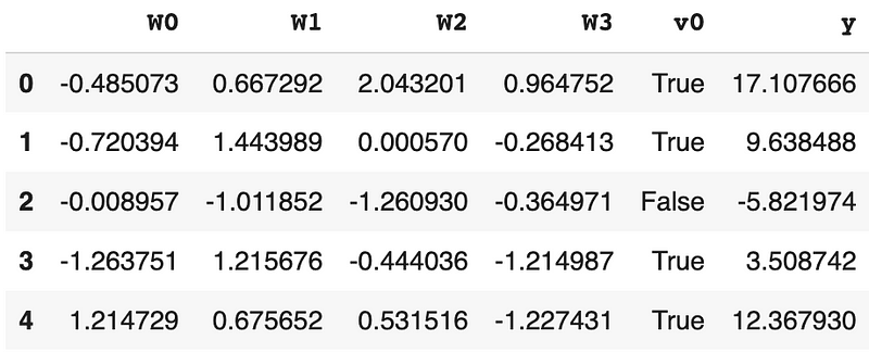
Next, let’s rename v0 to treatment, rename y to outcome, and convert the boolean values to 0s and 1s.
# Rename columns
df = df.rename({'v0': 'treatment', 'y': 'outcome'}, axis=1)
# Create the treatment variable, and change boolean values to 1 and 0
df['treatment'] = df['treatment'].apply(lambda x: 1 if x == True else 0)# Take a look at the data
df.head()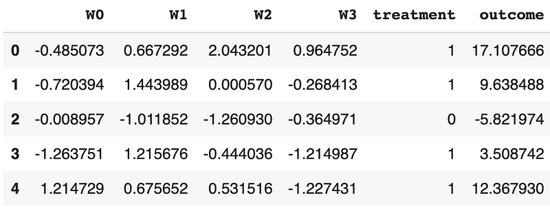
Finally, the Python dataframe is converted to R dataframe in order to use R packages on the dataset.
# Convert Python dataframe to R dataframe
with localconverter(ro.default_converter + pandas2ri.converter):
  dfr = ro.conversion.py2rpy(df)
# Create a variable name in R's global environment
from rpy2.robjects import globalenv
globalenv['dfr'] = dfrStep 3: Unadjusted Mean Differences Before Propensity Score Matching (PSM)
In step 3, we will get the unadjusted difference between the treatment group and the non-treatment group.
%%R
# Get the matched treatement outcomes
y_treatment <- dfr$outcome[dfr$treatment==1]
# Get the matched control outcomes
y_control <- dfr$outcome[dfr$treatment==0]# Get the mean difference
unadjusted_diff <- mean(y_treatment - y_control)
print(unadjusted_diff)If we do not use causal inference and take the direct difference between the two groups, we will conclude that the treatment increased the outcome by 16, which is much higher than the true causal impact of 10.
16.13221Step 4: Pre-Matching Standardized Mean Difference of Confounders
In step 4, we will check the standardized mean difference (SMD) between the treatment group and the non-treatment group.
var=confoundersmeans that we will summarize the data for the four confounders.strata='treatment'means that the variables will be grouped by the treatment type.test=TRUEmeans the p-value for the significance testing will be reported.smd=TRUEmeans that the standardized mean difference will be reported.
%%R
# Confounders
confounders <- c('W0', 'W1', 'W2', 'W3')
# Create table one, test=TRUE means with significance testing
table1 <- CreateTableOne(var=confounders, strata='treatment', data=dfr, test=TRUE)# Print the results
print(table1, smd=TRUE)Standardized Mean Differences(SMD) greater than 0.1 is usually used to check the imbalance between the treatment and the control group. We can see that most confounders have SMD greater than 0.1 with a significant p-value, meaning that the confounders differ between the treatment group and the non-treatment group.
Step 5: Propensity Score Matching (PSM) Using R Package MatchIt
In step 5, we will talk about how to use the R MatchIt package to do the Propensity Score Matching (PSM).
- The propensity score is the probability of getting the treatment, so we need to use the confounders to predict the probability of getting the treatment.
- method=’nearest’ means that we are using the nearest neighbor method. Nearest neighbor matching is a widely used greedy matching method. Greedy matching matches the nearest control at the moment, and removes the matched control from the rest of the matching. It’s fast but sensitive to the order of samples. It is not optimal to minimize the total distance because the samples matched later in the process cannot be matched with the controls that have been matched.
distance = 'glm'means that we are using the propensity score difference to conduct the nearest neighbor matching. The default is to match from the highest to the lowest propensity score in the treatment group. This ensures the datapoint that is hard to get a match to be matched first.- ratio=1 means that one treatment unit is matched with one control unit. When the ratio is greater than 1, more than one control unit will with matched with each treatment unit. If we would like to have 2 controls matched for each treatment unit, the nearest neighbor matching will be executed for all the units in the treatment group to get the first match, then the process is repeated to get the second match. When there is a tie in propensity score, the one with the higher order in the dataset will be picked. This ensures the reproducibility of the results.
replace=Fmeans that each sample in the control group is only matched with one sample in the treatment group.- A caliper is the distance threshold for any match. The matched pairs with a distance greater than the caliper distance will be dropped.
caliper=.2means that matches greater than 20% of the standard deviations of propensity score will be dropped.
%%R
# Propensity score matching using matchit
psm_matchit <- matchit(treatment ~ W0 + W1 + W2 + W3, method='nearest', distance = 'glm', ratio=1, replace=F, caliper=0.2, data=dfr)
Step 6: Matched Dataset Balance Checking
In step 6, we will check the balance of the matched dataset from Propensity Score Matching (PSM). un = FALSE means that the balance summary for the dataset before matching will not be displayed. This is because we already have the pre-matching balance check in step 4.
%%R
# Check balance
summary(psm_matchit, un = FALSE)
We can see that 852 units in the treatment group found matches in the control group. The standardized mean difference (SMD) decreased for every confounder. Three of the four confounders have the standardized mean difference (SMD) under 0.1 after Propensity Score Matching (PSM).
Call:
matchit(formula = treatment ~ W0 + W1 + W2 + W3, data = dfr,
    method = "nearest", distance = "glm", replace = F, caliper = 0.2,
    ratio = 1)
Summary of Balance for Matched Data:
Means Treated Means Control Std. Mean Diff. Var. Ratio eCDF Mean
distance 0.5881 0.5403 0.2948 1.1726 0.0492
W0 -0.4646 -0.5606 0.0988 1.1593 0.0218
W1 0.4439 0.2544 0.2286 2.7730 0.0476
W2 0.3118 0.2554 0.0569 1.0740 0.0148
W3 0.1524 0.1507 0.0017 1.0204 0.0077
eCDF Max Std. Pair Dist.
distance 0.0915 0.2951
W0 0.0446 1.1005
W1 0.0857 0.7930
W2 0.0516 1.0996
W3 0.0258 1.0875Sample Sizes:
Control Treated
All 2269 7731
Matched 852 852
Unmatched 1417 6879
Discarded 0 0Next, let’s visualize the matched dataset.
In the jitter plot of the propensity score distribution, the x-axis is the propensity score.
We can see that the matched treated and control units have a similar distribution of propensity scores.
The unmatched treatment units are mostly units with high propensity scores, and the unmatched control units are mostly those with low propensity scores. This is expected because the propensity score measures the probability of getting treatment.
%%R
# Distribution of propensity scores
plot(psm_matchit, type='jitter')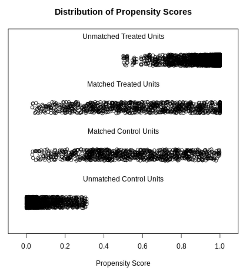
We can see the same distribution through a histogram plot. For the raw treated data, the propensity score for most units is quite high at more than 0.9, and for the raw control data, the propensity score for most units is quite low at less than 0.1.
The matched treatment and control groups have propensity score distributions much more similar than the raw data.
%%R
# Distribution of propensity scores
plot(psm_matchit, type='hist')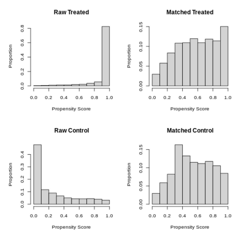
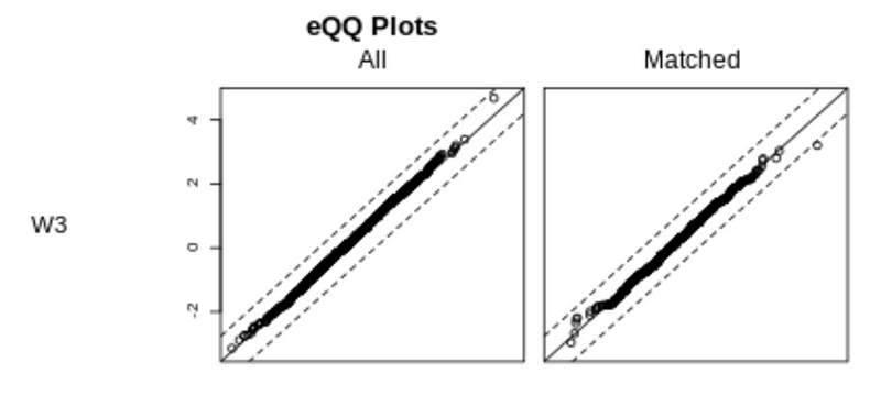
We can also visualize the balance check using a QQ plot. The diagonal line represents a balanced dataset.
For the covariates W0, W1, and W2, matching improved the balance of the dataset, but the covariate W1 is still not well balanced. This is consistent with the matched standardized mean difference (SMD) result that W1 is still above 0.1 after matching.
%%R
# QQ plot
plot(psm_matchit, type = "qq", interactive=FALSE)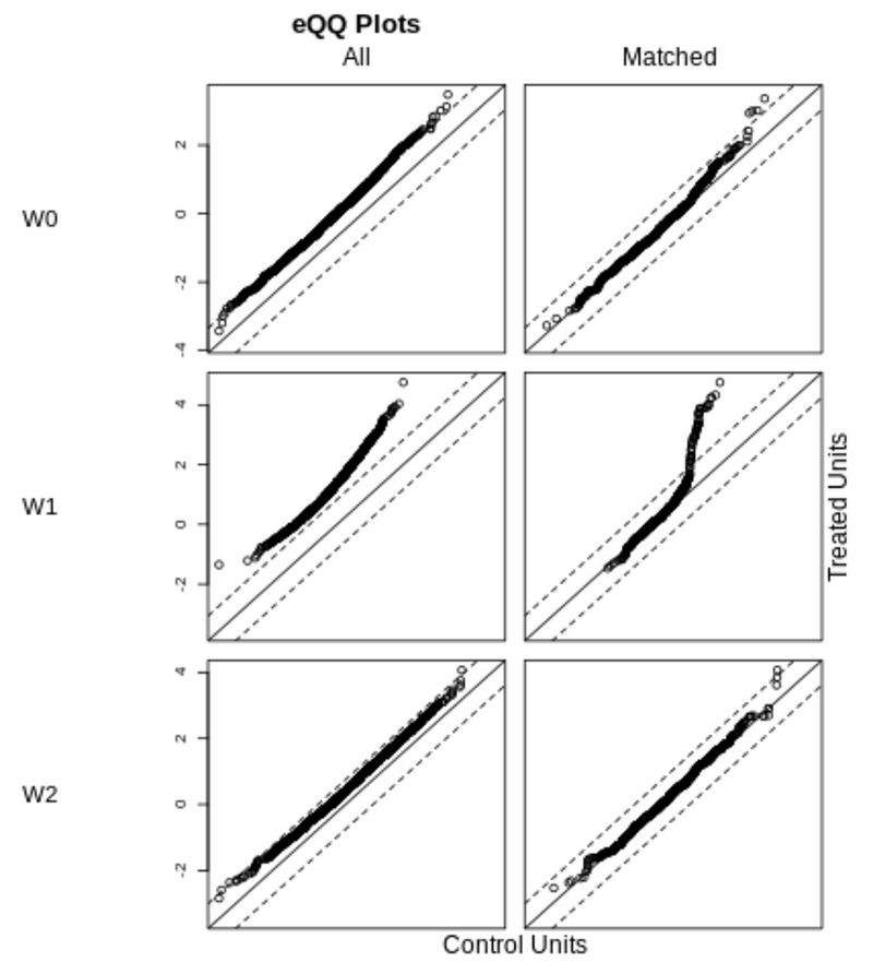
The covariate W3 is balanced both before and after matching, consistent with the results that the standardized mean difference (SMD) is below 0.1 before and after matching.
Using plot on the summary of the matchit output produces a Love plot.
From the Love plot, we can see that the Absolute Standardized Means Difference (SMD) decreased for all the covariates, and most of the matched results are under 0.1.
%%R
# Absolute Standardized Mean Difference
plot(summary(psm_matchit))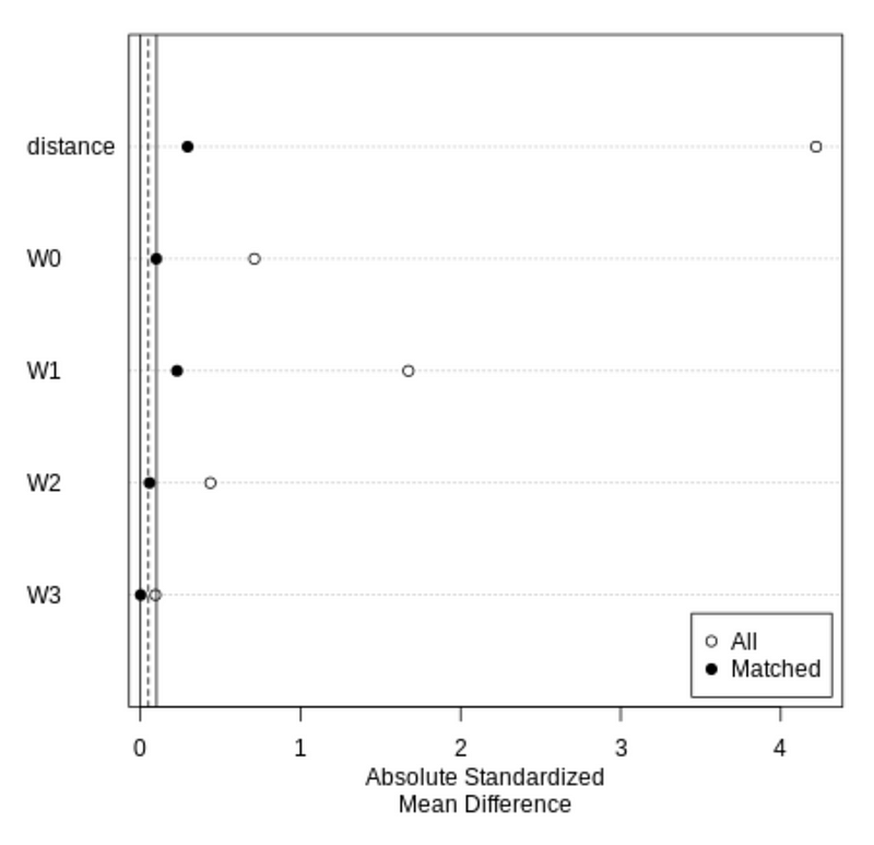
After assessing the balance of the matched data, we can assign the matched data to a variable and take a look at the matched dataset.
%%R
# Matched data
psm_matchit_data <- match.data(psm_matchit)
head(psm_matchit_data)
Output
W0         W1           W2         W3 treatment   outcome   distance
6  -0.8515585  0.6097349 -0.137718729  2.0495952         0  4.737745 0.77889637
7  -0.2644170 -0.1562823  1.286532796 -1.0235267         0 -1.725462 0.52742428
10 -1.7294418  0.1815844  0.003349113  1.2544392         1  8.844935 0.06776993
13 -1.0901373  0.5922162  0.795251315  1.1728621         1 13.082516 0.84158871
14 -0.7300940  0.7157696 -0.642347090 -0.9988897         0 -5.482522 0.61042180
18 -0.1638727  0.6024213  0.555748660 -1.7902519         1  6.080432 0.92796027
   weights subclass
6        1      721
7        1      297
10       1       12
13       1       39
14       1       30
18       1       89
Step 7: Estimating Treatment Effect Using T-Test
In step 7, we will estimate the treatment effect using a t-test.
The outcomes for the treatment and the control group are compared to see if there is a significant difference between the two.
%%R
# Get the matched treatement outcomes
y_treatment_psm_matchit <- psm_matchit_data$outcome[psm_matchit_data$treatment==1]
# Get the matched control outcomes
y_control_psm_matchit <- psm_matchit_data$outcome[psm_matchit_data$treatment==0]# t-test
t.test(y_treatment_psm_matchit,
y_control_psm_matchit,
var.equal = TRUE,
paired=FALSE,
conf.level=0.95)The outcome shows a p-value close to 0, indicating a significant difference between the treatment and the control group. The mean difference is 10.8, which is close to the true causal impact of 10, and much better than the unadjusted mean difference of 16.
Two Sample t-test
data:  y_treatment_psm_matchit and y_control_psm_matchit
t = 50.02, df = 1702, p-value < 2.2e-16
alternative hypothesis: true difference in means is not equal to 0
95 percent confidence interval:  10.37724 11.22427 sample estimates:
mean of x  mean of y
10.5164146 -0.2843384
Step 8: Estimating Treatment Effect Using Model
An alternative way is to estimate the treatment effect using a model.
In the model, the dependent variable is the outcome, and the independent variables are the covariates plus the treatment. The coefficient of the treatment variable is the causal impact.
%%R
# Model
model_psm_matchit <- lm(outcome ~ treatment + W0 + W1 + W2 + W3, data = psm_matchit_data, weights = weights)
# Coefficient test
coeftest(model_psm_matchit, vcov. = vcovCL, cluster = ~subclass)The output shows that the causal impact is 10, which is the same as the true causal impact, and more accurate than the unadjusted mean difference of 16.
t test of coefficients: Estimate Std. Error t value Pr(>|t|)
(Intercept) -0.00029029 0.00037869 -0.7665 0.4435
treatment 9.99991929 0.00048982 20415.6182 <2e-16 ***
W0 3.20571166 0.00025212 12714.8728 <2e-16 ***
W1 1.95359593 0.00034929 5593.0647 <2e-16 ***
W2 2.08778715 0.00025094 8319.7113 <2e-16 ***
W3 3.20370684 0.00024183 13247.8749 <2e-16 ***
---
Signif. codes: 0 ‘***’ 0.001 ‘**’ 0.01 ‘*’ 0.05 ‘.’ 0.1 ‘ ’ 1Summary
This tutorial talked about how to conduct causal inference propensity score matching (PSM) using R package MatchIt. You learned:
- How do the Propensity Score Matching (PSM) algorithms work?
- How to conduct Propensity Score Matching (PSM) using the R package MatchIt?
- How to check the balance of the matched dataset?
- How to calculate causal impact using a t-test or a regression model?
The results show that after propensity score matching (PSM), both the t-test and the regression model calculated the causal impact close to the true value, and the regression model has slightly better accuracy than the t-test.
More tutorials are available on GrabNGoInfo YouTube Channel and GrabNGoInfo.com.
Recommended Tutorials
- GrabNGoInfo Machine Learning Tutorials Inventory
- One-Class SVM For Anomaly Detection
- 3 Ways for Multiple Time Series Forecasting Using Prophet in Python
- Recommendation System: User-Based Collaborative Filtering
- Four Oversampling And Under-Sampling Methods For Imbalanced Classification Using Python
- Causal Inference One-to-one Matching on Confounders Using R for Python Users
- How to detect outliers | Data Science Interview Questions and Answers
References
[2] rpy2 R and pandas Dataframe Documentation
[3] Stuart EA. Matching methods for causal inference: A review and a look forward. Stat Sci. 2010 Feb 1;25(1):1–21. doi: 10.1214/09-STS313. PMID: 20871802; PMCID: PMC2943670.
[5] Coursera course: A Crash Course in Causality


