Causal Effects via DAGs

Breaking down the Back and Front Door Criteria

This is the 4th article in a series on causal effects. In the last article of this series, we explored the question of identifiability. In other words, can the causal effect be evaluated from the given data? There we saw a systematic 3-step process to express any causal effect given a causal model where all variables are observed. The problem, however, becomes much more interesting when we have unmeasured confounders. In this article, I discuss two quick-and-easy graphical criteria for evaluating causal effects.

Identifiability

Identifiability is a central question in causal analysis i.e. can the causal effect be evaluated from the given data? In the previous blog, we saw a systematic 3-step process for answering this question for so-called Markovian causal models. These causal models satisfy two conditions: 1) no cycles and 2) no unmeasured noise terms that simultaneously cause two or more variables. This type of model can be represented by a directed cyclic graph i.e. a DAG. Examples of Markovian and non-Markovian DAGs are shown below.

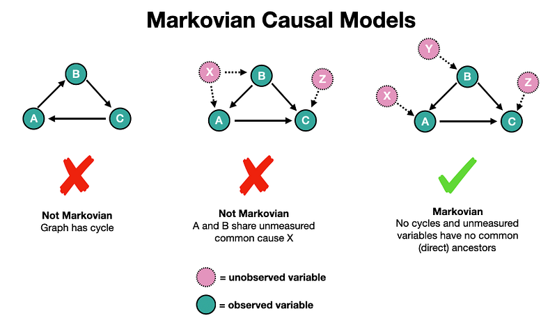
The Markov condition is important because it guarantees identifiability. In other words, if our causal model is Markovian, then the causal effect is always identifiable [1, 2]. While this is a powerful insight, it is also restrictive because we may be interested in causal models that are not Markovian.

For example, a Markovian model could become non-Markovian if there is an unmeasured confounder. We saw an example of this in the previous blog. The same example is shown in the figure below.

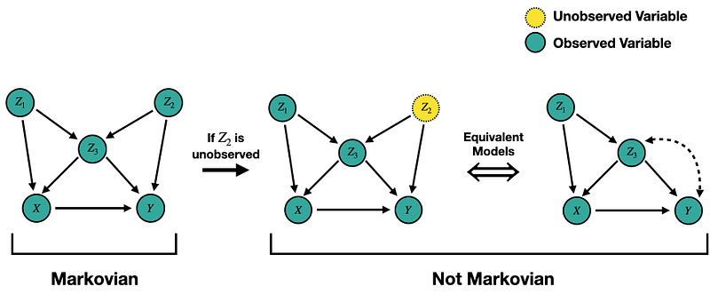
We start with the Markovian model on the far left. Then suppose Jimmy forgot to turn on the Z2 sensor, so we have no observations for the variable Z2. This situation is depicted by the model in the middle. Here we have an unobserved variable (Z2) with two children (Z3 and Y).

We can equivalently represent this situation by removing the unobserved variable from the DAG and connecting its two child nodes with a bi-directed edge [1]. Intuitively, the bi-directed edge represents the statistical dependence between Z3 and Y via Z2, but without observations of Z2, this will appear as a spurious association between the two in our data.

Note that the two right-most causal models are not Markovian. The middle one has an unmeasured noise term that simultaneously causes two variables, and the far right one has a cycle. Although these models are not Markovian, the causal effect of X on Y is indeed identifiable (more on that later).

3 Rules of Do-Calculus

In the general case, the question of identifiability can always be answered using the Rules of Do-Calculus [3, 4]. These are 3 rules we can use to manipulate interventional distributions—in other words, expressing probabilities that include the do-operator in terms of probabilities that do not include the do-operator.

A key point is that this set of rules is complete, which means that if identifiability cannot be established with these 3 rules, then the causal effect is not identifiable.

Rules of Do-Calculus — Given X, Y, Z, and W are arbitrary disjoint sets of variables in a causal model G, the Rules of Do-Calculus are given below.

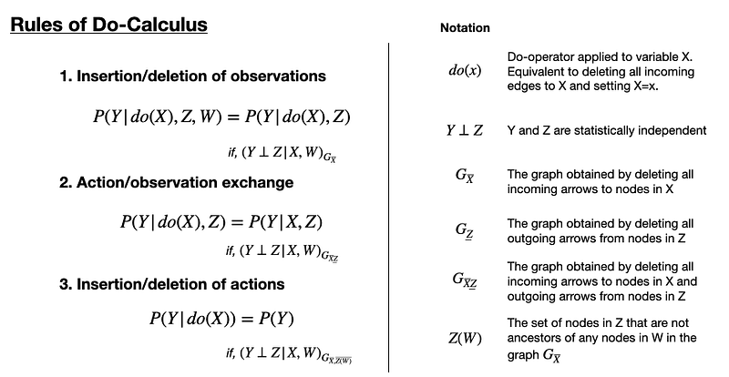
Although these rules are concise and complete, there is a lot to chew on here. For example, looking at rule 1, we can ignore the set of variables W only if Y and Z are conditionally independent in the graph obtained by deleting all the incoming arrows to the nodes in X.

Without a strong intuition for these rules and associated concepts, applying them to problems can be slow and challenging. That is where two quick and easy tests for identifiability can help.

2 Quick-and-Easy Graphical Criteria

While the Rules of Do-Calculus give us a complete set of operations for evaluating causal effects, using them in practice can be difficult for complicated DAGs. To help with this difficulty, we can turn to 2 practical graphical criteria for evaluating identifiability: the Back Door Criterion (BDC) and the Front Door Criterion (FDC).

Unlike the rules of do-calculus, these criteria are not complete. Meaning even if they are not satisfied, the causal effect may still be identifiable. Their key utility, however, is they serve as practical tests we can readily apply to answer causal questions before resorting to the Rules of Do-Calculus.

1) Back Door Criterion

The Back Door Criterion (BDC) is a relatively quick-and-easy test to evaluate if a set of nodes is sufficient to answer the question of identifiability. In other words, it tells us what variables we need to measure to calculate a particular causal effect.

Before defining the BDC, we first must arm ourselves with two key concepts: a back-door path and blocking.

A back-door path between 2 nodes (say X and Y) is any path that starts with an arrow pointing into X and terminates at Y [3]. For example, these are all the back door paths in the graph below.

• X <- Z1 -> Z3 -> Y
• X <- Z1 -> Z3 <- Z2 -> Y
• X <- Z3 -> Y
• X <- Z3 <- Z2 -> Y

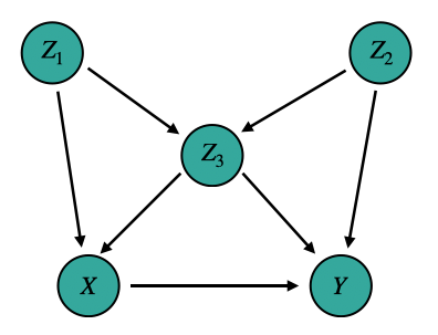
Notice that we ignore the arrowheads when constructing back-door paths (except, of course, for the one pointing into X). The intuition behind back door paths is they carry spurious associations between 2 variables [2].

The 2nd key concept here is that of blocking [3]. A path p is said to be blocked by a set of nodes {Z_i} if and only if,

1. p contains a chain A -> B -> C or a fork A <- B -> C, such that B is an element in {Z_i} — This is what we might intuitively think of as blocking
2. p contains a collider (i.e. an inverted fork) A -> B <- C, such that B and any of its descendants are not in {Z_i} — No node in {Z_i} creates a spurious statistical association (Berkson’s Paradox)

We can now combine these concepts to define the back door criterion [3].

Back Door Criterion — A set of nodes {Z_i} satisfy the BDC relative to (X, Y) if,

1. No node is a descendant of X (i.e. {Z_i} exclusively sit in back-door paths)
2. {Z_i} blocks every back door path between X and Y

Applying the BDC to the above graph, we can see that three sets of nodes satisfy this criterion [2].

• {Z1, Z3}
• {Z2, Z3}
• {Z1, Z2, Z3}

Notice the set {Z3} does not satisfy the BDC because it is a collider and thus does not satisfy our definition of blocking from before.

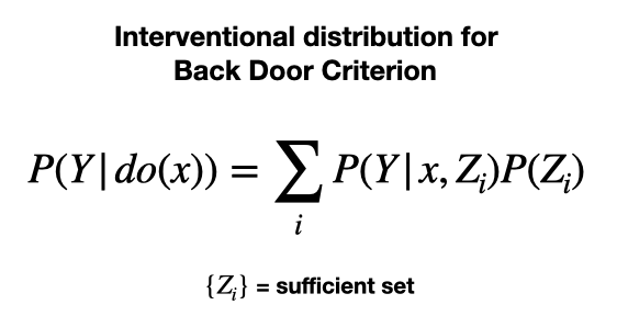
The sets {Z1, Z3}, {Z2, Z3}, and {Z1, Z2, Z3} are called sufficient sets (also admissible sets). They tell us which variables to measure to calculate unbiased causal effects between X and Y. We can express the interventional distribution using the following equation whenever the BDC is satisfied.

Note on Propensity Score Methods

A key point connecting the back door criterion to the Propensity Score (PS) methods we saw in an earlier blog is Propensity Score methods fail when the back door criterion is not satisfied [2]. In other words, if the variables used to derive a propensity score do not make up a sufficient set, they may introduce bias into the causal effect estimate.

While one may (naively) think the more variables used in the PS model, the better, this can backfire [5]. In some cases, like with variable Z3 in the above DAG, including particular variables may increase propensity score matching bias [2].

2) Front Door Criterion

Another quick-and-easy test we can use to evaluate identifiability is the Front Door criterion (FDC) [3]. A set of nodes {Z_i} satisfy the FDC relative to (X, Y) if

1. {Z_i} intercepts all directed paths from X to Y
2. All back door paths from X to {Z_i} are blocked by the empty set
3. All back door paths from {Z_i} to Y are blocked by X

Let’s look at another example. Consider the DAG below.

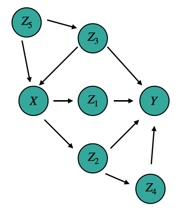
We can first seek a set of variables that satisfies condition 1. To do that, we enumerate all the directed paths from X and Y. In this case, there are only 3.

• X -> Z1 -> Y
• X -> Z2 -> Y
• X -> Z2 -> Y

From this, we can see {Z1, Z2} satisfies condition 1. But we aren’t done yet. We need to check whether this set satisfied the FDC by checking it against conditions 2 and 3.

To check condition 2, we need to look at all the back door paths from X to every node in {Z1, Z2}.

X and Z1

• X <- Z3 -> Y <- Z1
• X <- Z5 -> Z3 -> Y <- Z1

X and Z2

• X <- Z3 -> Y <- Z2
• X <- Z5 -> Z3 -> Y <- Z2
• X <- Z5 -> Z3 -> Y <- Z4 <- Z2

We can see that all these paths are blocked because they include a collider Y.

Then finally, we check condition 3 by looking at all the back door paths between every variable in {Z1, Z2} and Y.

Z1 and Y

• Z1 <- X <- Z3 -> Y
• Z1 <- X <- Z5 -> Z3 -> Y
• Z1 <- X -> Z2 -> Y
• Z1 <- X -> Z2 <- Z4 -> Y

Z2 and Y

• Z2 <- X <- Z3 -> Y
• Z2 <- X <- Z5 -> Z3 -> Y
• Z2 <- X -> Z1 -> Y

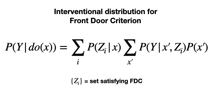
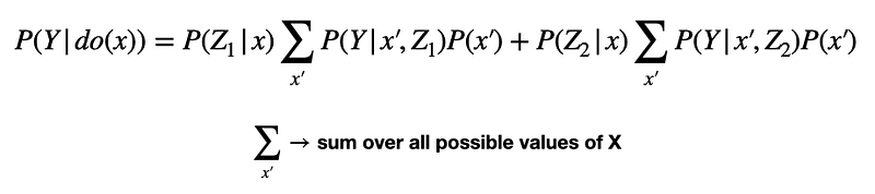
And indeed, we see that all these paths are blocked by X. Thus, we conclude that in order to estimate the causal effect of X and Y, we need only measure variables X, Y, Z1, and Z2. We can do this using the equation below, which expresses the interventional distribution P(Y|do(x)) in terms of observational distributions, including X, Y, Z1, and Z2

Notice for each variable in {Z_i}, we sum over all possible values of variable X. Writing things out a little more explicitly for the above example we have.

Key Points:

• Identifiability is concerned with answering the question: can the causal effect be evaluated from the given data?
• The 3 Rules of Do-Calculus gives us a complete set of operations to evaluate identifiability.
• We can also evaluate identifiability via two quick-and-easy graphical tests: the Back Door Criterion and the Front Door Criterion.

What’s next?

👉 More on Causality: Causal Effects Overview | Causality: Intro | Causal Inference | Causal Discovery

Resources

Connect: My website | Book a call | Ask me anything

Socials: YouTube 🎥 | LinkedIn | Twitter

Support: Buy me a coffee ☕️

[1] Tian, J., & Pearl, J. (2002). A General Identification Condition for Causal Effects. Proceedings of the Eighteenth National Conference on Artificial Intelligence. www.aaai.org

[2] Pearl, J. (2010). The International Journal of Biostatistics: An Introduction to Causal Inference. The International Journal of Biostatistics, 6(2), Article 7. https://doi.org/10.2202/1557-4679.1203

[3] Tian, J., & Shpitser, I. (n.d.). On Identifying Causal Effects.

[4] Pearl, J. (2012). The Do-Calculus Revisited. Proceedings of the Twenty-Eight Conference on Uncertainty in Artificial Intelligence, August, 4–11. http://arxiv.org/abs/1210.4852

[5] Pearl, J. (2009). Myth, Confusion, and Science in Causal Analysis.