
Case Study #3: Netflix Subscription Forecasting — Resume Project
A Guide to a Resume-worthy Data Science Project
On the 15th of October, it was a Sunday morning, and I was brewing my morning coffee. I normally start my mornings with coffee in my hand, reading emails, and doing business works. However, I was scrolling through my Instagram feed that morning since I wasn’t in the mood for any professional work. Then I came upon this case study in one of the data science influencers’ posts. Then I decided to tackle a fun activity and take a break from business for the day. I, on the other hand, prefer working on small data science projects. So, as you already know, the project I worked on was “Netflix Subscription Forecasting.”
The goal of this case study was to forecast the number of subscribers for the following quarters. As a result, it will help in optimizing its resource planning based on the forecasted outcome.
Initial Thought:
I went over the data when I originally received the dataset for the case study. It just featured two columns: “Time Period” and “Number of Subscribers”. The “time period” was given in quarters. So it was evident to me that I needed to anticipate the number of subscribers for the following eight quarters, and I believed it would be a simple task, and I was eager to get my hands dirty with the project.
Data Exploration:
I began by loading the dataset into a DataFrame. Then I began studying the data by looking for missing numbers, outliers, and the structure of the data. And discovered that “Time Period” was not in “datetime” format, which is required for any time series analysis.
import pandas as pd

df = pd.read_csv('Netflix-Subscriptions.csv')
df.head()

df.isnull().sum()

df.describe()

df.info()
Data Preparation:
So my first technical task was to convert the “Time Period” column to a datetime format, set it up as a DataFrame index, and sort the data chronologically. It will prepare the data for any time-series modeling techniques that I will apply to it later.
df['Time Period'] = pd.to_datetime(df['Time Period'])
df.set_index('Time Period', inplace = True)
df.sort_index(inplace = True)
Time-Series Decomposition:
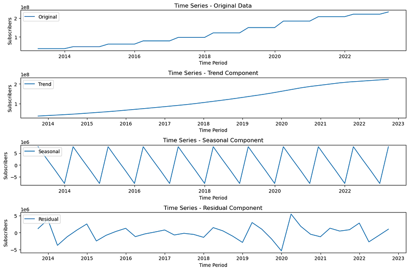
I considered conducting “time-series decomposition” before diving into modeling. “What is that?” you may wonder. In simple terms, it is a method that breaks down data into trend, seasonal, and residual components, allowing us to better understand the underlying patterns in the data.
Also, before decomposing the data, I resampled it because the data was in irregular time intervals, and time-series analysis requires equispaced data for better results.
import matplotlib.pyplot as plt
from statsmodels.tsa.seasonal import seasonal_decompose

df_resampled = df.resample('Q').mean().ffill()
df_resampled.index.freq = 'Q'

#Decomposition Starts here...
decomposition = seasonal_decompose(df_resampled['Subscribers'], model = 'additive')

#Visualizing trends, seasonality, etc. after decomposing...
plt.figure(figsize =(12,8))

plt.subplot(411)
plt.plot(df_resampled['Subscribers'], label = 'Original')
plt.legend(loc = 'upper left')
plt.title('Time Series - Original Data')
plt.xlabel('Time Period')
plt.ylabel('Subscribers')

plt.subplot(412)
plt.plot(decomposition.trend, label = 'Trend')
plt.legend(loc = 'upper left')
plt.title('Time Series - Trend Component')
plt.xlabel('Time Period')
plt.ylabel('Subscribers')

plt.subplot(413)
plt.plot(decomposition.seasonal, label = 'Seasonal')
plt.legend(loc = 'upper left')
plt.title('Time Series - Seasonal Component')
plt.xlabel('Time Period')
plt.ylabel('Subscribers')

plt.subplot(414)
plt.plot(decomposition.resid, label = 'Residual')
plt.legend(loc = 'upper left')
plt.title('Time Series - Residual Component')
plt.xlabel('Time Period')
plt.ylabel('Subscribers')

plt.tight_layout()
plt.show()
After decomposing the data, I observed a trend as well as seasonality. So, my initial modeling approach was that a seasonal model would be appropriate for this data.
Hey, Sorry for interrupting, but if you have enjoyed the story so far and are feeling generous, you can support me by giving me a “Tip” as I am unable to join in MPP because of the location. barrier.
Model Selection:
As I previously stated, I noticed a trend and seasonality in the data. Hence, I considered utilizing the SARIMA (Seasonal ARIMA) model for this project. But don’t be worried! As a backup, I considered using the ARIMA model to evaluate how big of a difference seasonality makes.
Model Training:
This is the tough part. Training a SARIMA model is a difficult task. It contains several hyperparameters (p,d,q), and selecting the proper combination is crucial since it has a significant influence on the model’s performance. As a result, I chose to do a grid search to determine the best set of hyperparameters based on the AIC (Akaike Information Criterion). Here, a lower AIC normally indicates a better model fit, but it was imperative to balance this with the model’s complexity to avoid overfitting.
from statsmodels.tsa.statespace.sarimax import SARIMAX
from itertools import product
import warnings
warnings.filterwarnings('ignore')

#Hyperparameter Tuning for SARIMA:
p = d = q = range(0,2)
pdq = list(product(p,d,q))


seasonal_pdq = [(x[0], x[1], x[2], 4) for x in pdq]

best_aic = float("inf")
best_pdq = None
best_seasonal_pdq = None

for param in pdq:
    for param_seasonal in seasonal_pdq:
        try:
            model = SARIMAX(df_resampled['Subscribers'],
                          order = param,
                          seasonal_order = param_seasonal,
                          enforce_stationarity = False,
                          enforce_invertibility = False)
            results = model.fit()
            if results.aic < best_aic:
                best_aic = results.aic
                best_pdq = param
                best_seasonal_pdq = param_seasonal
        except:
            continue

best_aic, best_pdq, best_seasonal_pdqOutput: (972.8543051925668, (0, 1, 1), (1, 1, 1, 4))Finally, I got the optimal hyperparameters, and once acquired, I fitted the SARIMA model and examined the diagnostic plots to check that the model’s residuals behaved as I expected.
best_model = SARIMAX(df_resampled['Subscribers'],
                    order = best_pdq,
                    seasonal_order = best_seasonal_pdq,
                    enforce_stationarity= False,
                    enforce_invertibility= False)
best_results = best_model.fit()

best_results.plot_diagnostics(figsize = (15, 12))
plt.show()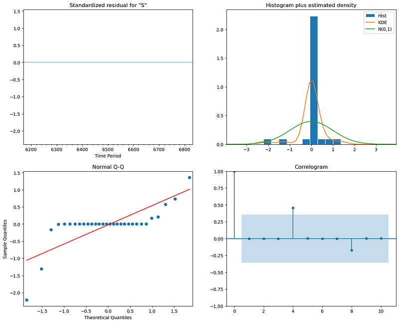
Forecasting:
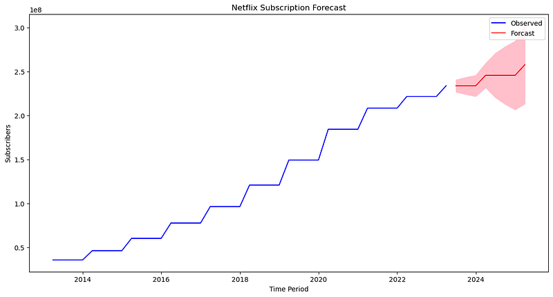
With everything in order and the SARIMA model in place, I forecast the following eight quarters and plotted them with a confidence interval to offer viewers or readers (company stakeholders) a notion of forecasting uncertainty.
Finally, I ran an ARIMA model using a similar grid search approach. SARIMA was the best model after comparing the AICs, confirming my initial hunch regarding the seasonality in the data.
forecast = best_results.get_forecast(steps = 8)
mean_forecast = forecast.predicted_mean
confidence_intervals = forecast.conf_int()

plt.figure(figsize = (14,7))
plt.plot(df_resampled.index, df_resampled['Subscribers'], label = 'Observed', color = 'b')
plt.plot(mean_forecast.index, mean_forecast, label ='Forcast', color = 'r')
plt.fill_between(confidence_intervals.index,
                confidence_intervals.iloc[:,0],
                confidence_intervals.iloc[:, 1], color = 'pink')
plt.xlabel('Time Period')
plt.ylabel('Subscribers')
plt.title('Netflix Subscription Forecast')

plt.legend()
plt.show()

#The Forecasted graph is shown at the beginning of the story.
#Here, have a look at it again...Full Project Link: https://github.com/richardwarepam16/Netflix-Subscription-Forecasting-Using-SARIMA/blob/master/SubscriptionNotebook.ipynb
Conclusion:
As a conclusion to this story, this is how I completed the case study in less than an hour, simply for fun playing with the data. Also, these are the results: Model Evaluation: ARIMA AIC: 1409.59 and SARIMA AIC: 972.60 Forecasted Results: By the end of Q1 2025, the number of subscribers is estimated to reach around 2.56 x 10⁸. Recommendations: 1. Given its forecasted growth, I would recommend scaling resources proportionately. 2. In addition, given the history of continued growth, I would propose offering an opportunity to introduce new features or strategies for marketing. Finally, this is all I accomplished in this case study, but you may continue by fine-tuning the model and adding more data points to create a more thorough model. Best of luck!👍
If you really enjoyed this article,
- Please subscribe to my new newsletter to get weekly programming tips and tech trends: “AI CodeHub Newsletter.”
- Please clap on this story and also,
- Highlight your favorite part of this story.
- ⭐️ Click here, You can also buy me a coffee if you like this story. It will be a great help to me. Thank You!
- Lastly, follow me for more technical blogs, ebooks, and case studies: Link


