Click to navigate: Part 1 -> Part 2 -> Part 3

Segmenting Abnormalities in Mammograms (Part 3 of 3)

A step-by-step guide to implementing a deep learning semantic segmentation pipeline on mammograms in TensorFlow 2

If you are reading this article, chances are that we share similar interests and are in similar industries. So let’s connect via LinkedIn, where I share tidbits of my thoughts and resources about AI and ML!

Article Structure

This article is Part 3 of a 3-part series that walks through how I tackled a deep learning project of identifying mass abnormalities in mammogram scans using an image segmentation model. As a result of breaking down the project in detail, this serves as a comprehensive overview of one of the core problems in computer vision — semantic segmentation, as well as a deep dive into the technicalities of executing this project in TensorFlow 2.

Part 1:

• Problem statement.
• What is semantic segmentation.
• Guide to downloading the dataset.
• What you’ll find in the dataset.
• Unravelling the nested folder structure of the dataset.
• Data exploration.

Part 2:

• Image preprocessing pipeline overview.
• General issues with the raw mammograms.
• Deep dive into raw mammogram’s preprocessing pipeline.
• Deep dive into corresponding mask’s preprocessing pipeline.

Part 3:

• Introducing the VGG-16 U-Net model.
• Implementing the model in TensorFlow 2.
• Notes on training the model.
• Results and post analysis.
• Wrapping up.

GitHub Repository

The code for this project can be found on my Github in this repository.

Continuing From Part 2

We ended Part 2 with an in-depth understanding of our image preprocessing pipeline, as well as reusable code for each image preprocessing step. With the pipeline, we were able to progress from the raw images to preprocessed images that can be fed into a segmentation model.

In this part, we cover the intuition behind the chosen segmentation model (VGG-16 U-Net), how to implement it in Tensorflow 2 and also evaluation of the results.

1. Introducing the VGG-16 U-Net Model

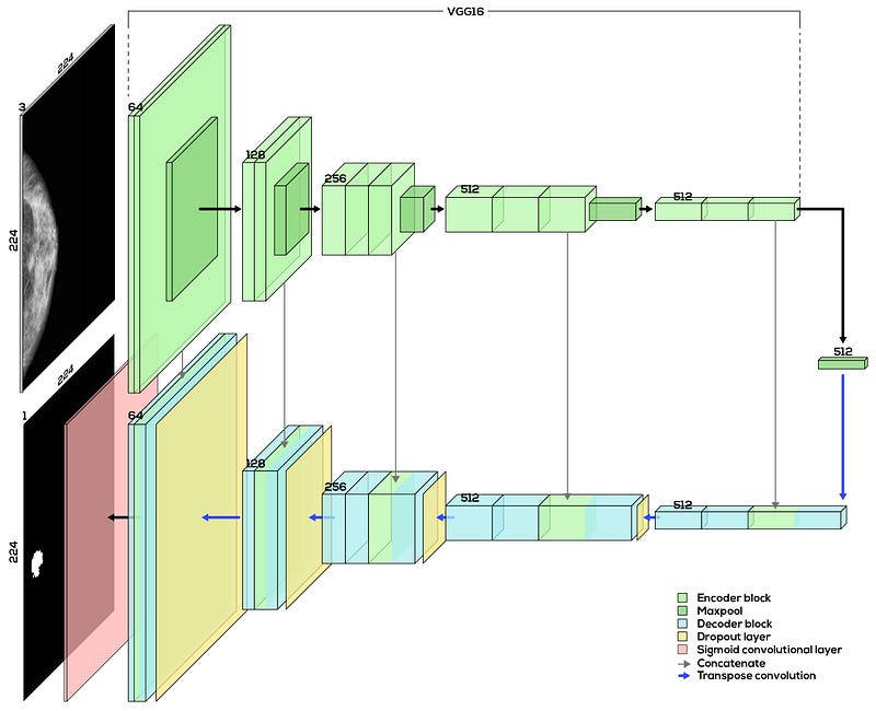
Since Olaf Ronneberger et al. developed and documented the U-Net architecture in the release of his paper “U-Net: Convolutional Networks for Biomedical Image Segmentation” in 2015, the U-Net has become a common architecture used for segmentation tasks. It comprises two main parts — the encoder block (top half of the diagram) and the decoder block (bottom half of the diagram). These two parts together form a U-shape when illustrated, which explains its name.

The high-level intuition of what a U-Net does is as such. The encoder block learns features and tells us “what is in the image”, just like it would in a classification task. The decoder block then semantically projects these low-resolution features learnt by the encoder block back up to the full-resolution pixel space of the original input image, giving us a full-resolution segmentation map.

Encoder block: It is usually a traditional sequence of convolutional layers and max-pooling layers. Think of it as a typical convolutional neural network (CNN) architecture used for classification tasks but without the final dense layers (these type of networks are called Fully Convolutional Network (FCN)). This FCN can be of your own design, or it can be taken from any pre-existing CNNs like the AlexNet, VGG-16 or the ResNet. For this task, I have chosen the VGG-16 for the encoder block (without the final dense layers) because I understand it better than the other CNN models.

Decoder block: It is a network of upsampling convolutions and concatenation layers that is symmetric to the encoder block. As seen from Fig. 1, selected feature maps from the encoder block are concatenated to their corresponding layers in the decoder block. Since the earlier layers of CNNs tend to learn low-level features while later layers learn more high-level features, this concatenation allows the U-Net to map features learnt across all levels into producing the final full-resolution, predicted segmentation map.

I strongly recommend you read this article to get a more in-depth explanation of the U-Net architecture.

2. Implementing the Model in Tensorflow 2

import tensorflow as tf

from tensorflow import keras

In the actual code, I implemented the model as a Python class object called unetVgg16. For the sake of brevity, I only included parts of the code below that are essential to the implementation. You should visit the project’s repository for the full code that implements the model.

The function buildEncoder() is used to build the encoder part of the U-Net with the help of transfer learning. In lines 3 to 8, I imported the VGG-16 model with weights pre-trained on the ImageNet dataset from the Keras model zoo. Setting include_top=False removes the dense layers from VGG-16 that we do not want (the dense layers are considered the top layers in Keras), leaving us with only the FCN part of the VGG-16. If you are unfamiliar with transfer learning, this article should give a nice, gentle introduction to it.

The function buildUnet() then builds the decoder and consequently the entire U-Net architecture. It calls the buildEncoder() function to create the encoder block and builds the decoder block on top of it to eventually form the full architecture of the VGG-16 U-Net. As seen in Fig. 1, there are 5 main sub-blocks in the decoder block with Block 5 starting from the right of the diagram, followed by the final convolutional layer to the left (in red).

Since the buildUnet() function contains almost 300 lines of code (because it contains doc strings, comments and line breaks), you can refer to the repository here for the full code. When looking through the code, it is important to keep the following points in mind:

• keras.layers.Conv2D() builds the traditional convolutional layer.
• keras.layers.Dropout() inserts the traditional dropout layer.
• keras.layers.Concatenate() executes the concatenation at the start of each sub-block.
• keras.layers.Conv2DTranspose() is responsible for the upsampling of the feature map between each sub-block. This is what projects the low-resolution feature maps learnt by the encoder block to the full-resolution pixel space of the original image.

3. Notes on Training the Model

Now that we have properly preprocessed the images (from Part 2) and built the model, it is time to train the model.

I’d like to focus on two aspects of the training pipeline that are crucial and unique to this segmentation task — image augmentation and creating a custom IOU metric to be tracked at the end of every training epoch.

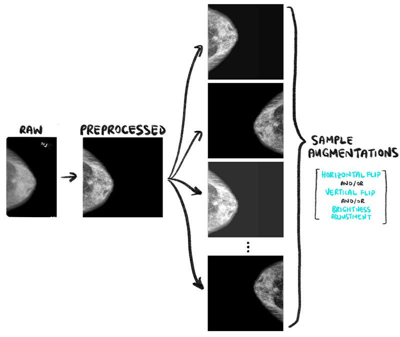
3.1. Image augmentation

Image augmentation can be used to artificially create new training data from existing training data and also to introduce variability in the dataset.

There are many image augmentations that can be done, of which I have chosen the following to perform:

1. Random horizontal flip (with 50% probability).
2. Random vertical flip (with 50% probability).
3. Random brightness adjustment.

If you wish to read up more about the other possible image augmentations in TensorFlow, this article is a good place to start.

The code snippet below shows how the random horizontal flips, vertical flips and brightness adjustments can be done in TensorFlow 2. As always, you can refer to the project’s repository for the full code.

We have to bear in mind that only the appropriate image augmentations can help with our model’s learning! When choosing the suitable augmentations, one of the most important considerations is the augmentations have to actually produce realistic images that are meaningful to our task.

What then are unrealistic and unmeaningful images that can result from inappropriate augmentations? Fig.3 illustrates a few examples of the results of doing random rotations, shears, width shifts and height shifts to the preprocessed mammograms.

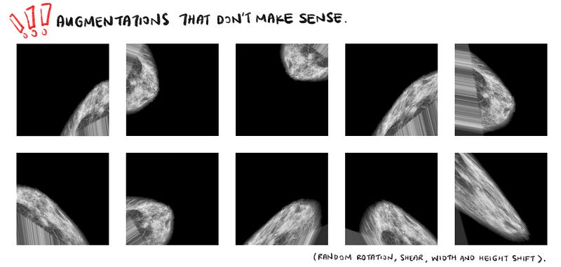
The above images are unrealistic and unmeaningful because we will almost never encounter such mammograms in reality! When we feed such senseless images into our model, the model will learn features that are not meaningful to the segmentation problem and slow down its convergence. Also bear in mind that these shears, rotations and shifts have to be applied to the masks as well, which is also very unrealistic and senseless.

In other words, when choosing the right image augmentations to perform, we have to ask ourselves, “Does augmenting the images this way make sense?”

3.2. Creating custom IOU metric

TensorFlow allows us to track certain metrics at the end of each training epoch through the metrics argument in the compile API. Typically, we use metrics like accuracy, precision and mean squared error. However, those metrics are not very applicable for semantic segmentation problems. Instead, the Intersection-Over-Union (IoU) metric is more commonly used.

Simply put, the IoU is the percentage overlap between the predicted segmentation and the ground truth, divided by the area of union between the predicted segmentation and the ground truth. This is better explained using the illustration in Fig. 4 below.

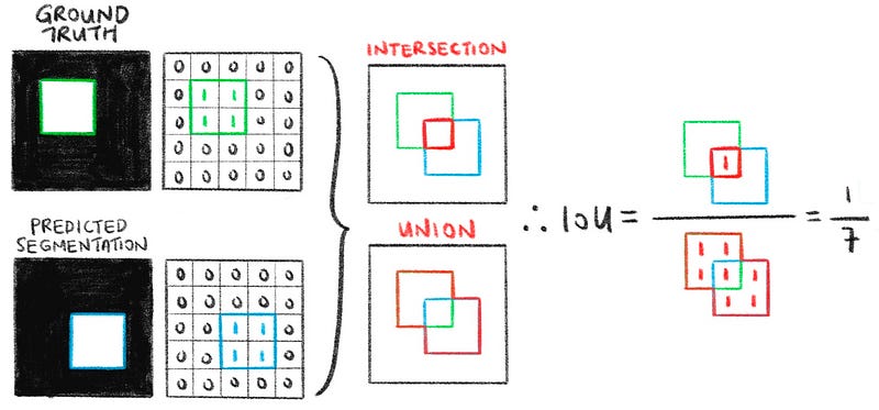
From the illustration, we see that IoU ranges from 0 to 1; 0 when the predicted segmentation is completely off (i.e. does not intersect with the ground truth at all) and 1 when the predicted segmentation exactly matches the ground truth. I strongly suggest reading the section titled “Why do we use Intersection over Union” in this article to better understand this metric.

The code snippet below shows how to implement the IoU in TensorFlow. Refer to the entire code here to see how I implemented it in TensorFlow’s compile API.

3.3. Training the model

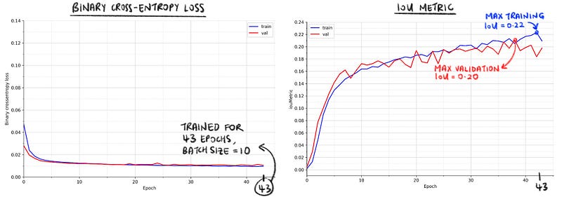
Finally, the model was trained under the following configurations and Fig. 5 above shows the training results.

• Number of epochs: 43 (stopped by Keras’ EarlyStop)
• Batch size: 10
• Learning rate: 0.00001
• Dropout rate: 0.5
• Loss function: Binary cross-entropy loss
• Optimiser: Adam

The maximum training and validation IoUs were around 0.20.

4. Results and Post Analysis

In this final section of the article, we dive deep into analysing the model’s predicted segmentations (a.k.a predicted masks). Since not many literature have been done on this specific segmentation problem, there are no benchmarks available to us for comparison. As such, we will be visually inspecting the masks and using a “first principles” approach to give a heuristic and logical evaluation of the results.

4.1. Analysing the predicted masks

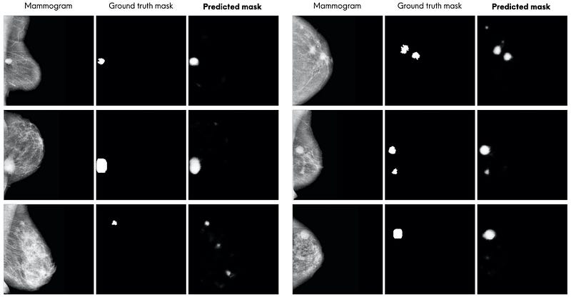
By a quick visual inspection, the predicted segmentations look quite accurate (note that “quite accurate” will be more formally defined in Section 4.4). The model is able to segment most of the mass abnormalities. It seems like the model’s main mistake is segmenting more regions than what are present in the ground truth masks (as opposed to segmenting less). Typically, these additional regions are bright spots in the mammograms and look very much like mass abnormalities.

Notice that the model’s predicted masks are soft masks (as opposed to a hard binary mask like the ground truth mask in the dataset). This is due to the final sigmoid layer of the U-Net causing the values in the predicted mask to range between 0.0 and 1.0. These pixel values can be interpreted as the probability of each pixel belonging to the “abnormality” class (1.0 representing certainty that the pixel is an abnormality).

4.2. Is IoU of 0.2 necessarily bad? Not really.

While the predicted segmentations generally look acceptable, it is natural to look at the IoU graph in Fig. 5 and ask, “Why is the highest mean IoU of the training (and validation) epochs only around 0.20?” (other segmentation problems sometimes have IoUs north of 0.80).

Before we address the question, note that the soft masks produced by the model might cause the IoUs to be lower than if it were to be a hard mask. This is debatable, since creating a hard mask from the soft mask would require some binarisation technique like thresholding, which might then affect the IoU score. Nevertheless, the soft masks that the model outputs are something to keep in mind.

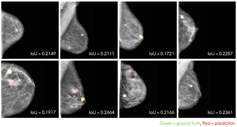
To address the question, it is more important to look at the predicted masks with IoUs around 0.20, as shown in Fig. 8 above, to see if they are acceptable. From these masks, we see that they are actually acceptable and not too different from the ground truth masks despite their low IoU scores. Also very importantly, the model is able to segment the nucleus of the mass abnormalities in most mammograms. In some mammograms, the model even segmented regions that indeed look like masses that the ground truth masks did not capture.

Hence, an average IoU of around 0.20 is actually pretty good for our particular segmentation problem, and a possible explanation for this low IoU might be the soft mask that the model outputs.

4.3. Looking at the lowest IoUs

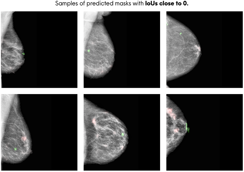
It is also important to look at the predicted masks with the lowest IoUs. Fig. 9 above shows that the model does not perform well at segmenting mass abnormalities when the abnormalities are very small, when the breast region has a web of dense breast tissues, or both.

4.4. Segmentation performance across the 3 most common mass shapes

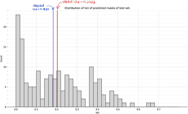
The three most common mass shapes in the dataset are lobulated, irregular and oval shape. We can get an idea of our model’s segmentation performance for each mass shape by looking at the percentage of “accurately” predicted masks for each mass shape.

What does accurately predicted mean? We can visually inspect the predicted masks to heuristically define what an “accurately predicted mask” is. To do that, we first visually inspect the predicted masks and identify ones that look accurate (i.e. looks very similar to the ground truth masks), then we use the IoUs of these masks to compute an “acceptable” IoU benchmark. Predicted masks that are above the benchmark can be deemed as “accurately predicted”.

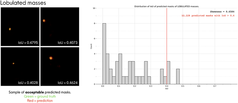
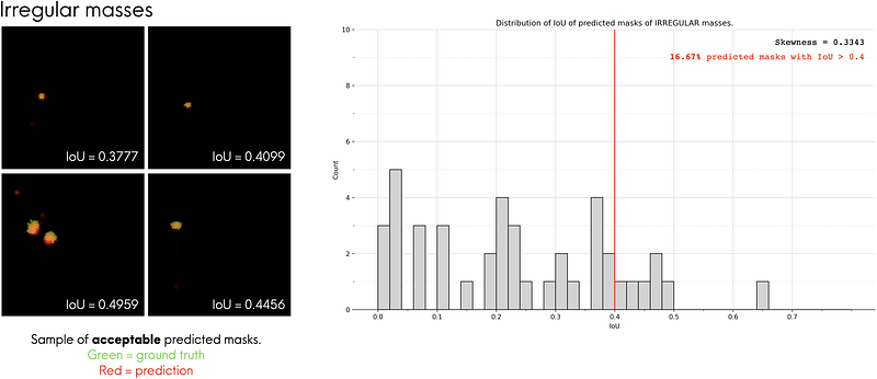
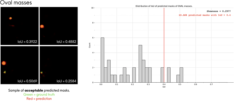
For each mass shape, I looked at the top 4 predicted masks that look the most similar to its corresponding ground truth masks and plotted them on the left of Fig. 10-a, 10-b and 10-c. I overlaid the predicted masks (red regions) and ground truth masks (green regions) to make them easier to compare. From there, we see that these predicted masks have IoUs of around 0.40. In other words, we can say that predicted masks that have an IoU ≥ 0.4 can be considered as accurate predictions. Using this benchmark, we see that the model performs the best for irregular-shaped masses, with 16.67% of them being predicted accurately by the model.

Wrapping Up

Finally, we have come to the end of this 3-part series, where we broke down the task of segmenting mass abnormalities from mammograms in great detail. In this series, you learnt what semantic segmentation is and how to build a pipeline for image segmentation tasks from start (downloading the data) to finish (evaluation of results). Most importantly, you learnt how I approached the problems faced at each stage of the pipeline and the intuition behind my code. You can now apply these mental frameworks to your own machine learning projects.

One last thing before you leave — here is the answer to the question in the title image throughout this series!

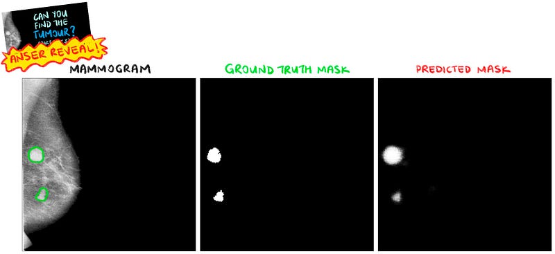
So… can you find the tumour?

You should check out Part 1 and Part 2 of this series if you haven’t, they give a nice background of the problem statement and gently builds up the knowledge needed to get the most out of Part 3!

Thank You

If you’ve made it to the end of this article, I hope that you enjoyed the read. If this article brought some inspiration, value or help to your own projects, feel free to share this with your community. Also, any constructive questions, feedback or discussions are definitely welcome, so please feel free to either comment down below or reach out to me on LinkedIn here or Twitter at @CleonW_.

Follow me on Medium (Cleon Wong) to stay in the loop for my next articles!