Can We Predict Performance of an NLP Model without Actually Training or Testing it?

An Alternative to Exhaustive Testing

Introduction:

Recently, Natural Language Processing has attracted a lot of research interest which has resulted in a number of models, tasks, datasets, etc. for numerous languages. This has lead to an explosion of experimental settings making it infeasible to collect high-quality test sets for each setting. Moreover, even for tasks where we do have a wide variety of test data( e.g. machine translation), it is still computationally prohibitive to build and test systems for all settings. Because of this, the common practice is to test new methods on a small subset of experimental settings. This impedes the community from gaining a comprehensive understanding of the newly-proposed approaches.

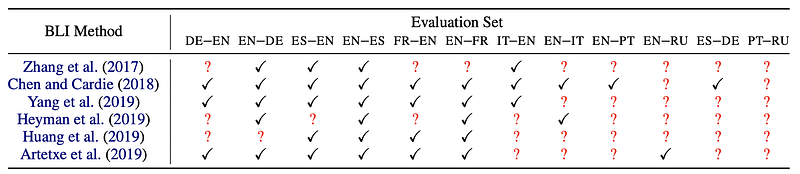
Table 1 illustrates this fact with an example from bilingual lexicon induction task (a task that aims to find word translation pairs from cross-lingual word embeddings). Almost all the works report evaluation results on a different evaluation set. Evaluating only on a small subset raises concerns about making inferences when comparing the merits of these methods. This motivates the problem of performance prediction i.e

Predicting how well a model can perform under an experimental setting without actually training or testing it.

Problem Formulation

Given a model M, which is trained over a training set D_tr based on a specific training strategy S, we then test the dataset D_ts under evaluation setting E and the test result y can be formulated as a function of the following inputs:

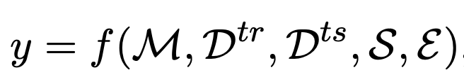
This is the actual performance, which requires us to run an actual experiment.

Performance Prediction requires us to calculate y, instead of performing a full training and evaluation cycle. Researchers estimate it by extracting features of M, D_tr, D_ts, S, and running them through a prediction function:

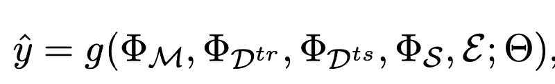
where Φ(·) represents features of the input, and Θ denotes learnable parameters. This is the predicted performance.

We expect y^ to give us a reasonable idea of experimental results much more efficiently than if we had to actually experiment.

NLPERF (Ref. 1)

They focus on dataset features(ΦL), language features (ΦD), and a single feature for the combination of the model architecture and training procedure (ΦC) to model the prediction function.

Concretely, they build regression models to predict the performance on a particular experimental setting given past experimental records of the same task, with each record consisting of the characterization of its training dataset and a performance score of the corresponding metric. i.e start with a partly populated table (such as Table 1) and attempt to infer the missing values with the predictor.

They experiment on a number of Tasks: Bilingual Lexicon Induction (BLI), Machine Translation, Cross-lingual Dependency Parsing (TSF-Parsing), Cross-lingual POS Tagging (TSF-POS), Cross-lingual Entity Linking (TSF-EL), Morphological Analysis (MA), Universal Dependency Parsing (UD).

Features Used for predictor model:

Language Features: They utilize six distance features from the URIEL Typological Database namely geographic, genetic, inventory, syntactic, phonological, and featural distance.

Dataset Features:

1. Training Dataset Size
2. Word/Subword Vocabulary Size
3. Average Sentence Length
4. Word/Subword Overlap:

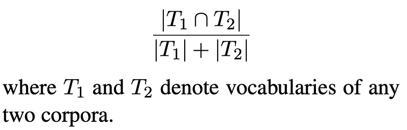
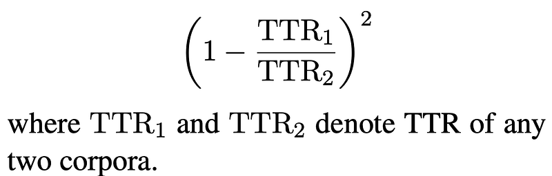
5. Type-Token Ratio (TTR): The ratio between the number of types and number of tokens of one corpus.

6. Type-Token Ratio Distance:

7. Single Tag Type: Number of single tag types

8. Fused Tag Type: Number of fused tag types.

9. Average Tag Length Per Word: Average number of single tags for each word.

10. Dependency Arcs Matching WALS Features: the proportion of dependency parsing arcs matching the following WALS features, computed over the training set: subject/object/oblique before/after verb and adjective/numeral before/after noun.

They use a subset of these features for different tasks. For instance, in the case of MT tasks, they use features 1–6 and language distance features.

Regression Model: They use gradient boosting trees (XGBoost) with squared error as the objective function for training the predictor.

Evaluation: k- fold cross validation i.e randomly partition the experimental records of ⟨L, D, C, S⟩ tuples into k folds, and use k−1 folds to train a prediction model and evaluate on the remaining fold. They use average root mean square error (RMSE) between the predicted scores and the true scores as the evaluation metric.

Performance Baselines:

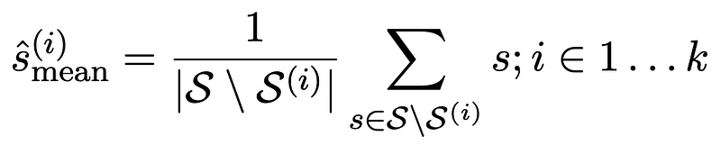
• Mean value baseline — outputs an average of scores s from the training folds for all test entries in the left-out evaluation fold (i) as follows:

They show that their approach outperforms these baselines. I intentionally omit the results here as this article is intended to present the motivation and the problem setup of this underexplored field.

Understanding Reliability of Performance Prediction Models (Ref. 2)

This work evaluates the reliability of performance prediction models from two angles:

1. Confidence Interval — Calculating confidence interval over performance predictions.
2. Calibration — Studying how well the confidence interval of prediction performance calibrates with the true probability of an experimental result.

Computing Confidence Interval: Refer to the Appendix below to get a basic understanding of confidence intervals. They sample K different training sets (with replacement) from the original training set and train K performance prediction models (1 model on each sampled training dataset) and evaluate K models on Φ(D)ts. This gives the distribution of predictions. Then, the confidence interval is computed based on the value of γ from this distribution (see appendix).

Calibration of Confidence Interval:

Note that confidence interval is calculated for the predicted performance yˆ, rather than the actual performance y, hence, it’s still unclear if the predicted CI is reliable enough to cover the actual performance. So, they try to answer the following question:

from an infinite number of independent trials, does the true value actually lie within the proposed intervals approximately 95% of the times?

To this end, they empirically examine the prediction distributions and establish the reliability of the confidence intervals. They compute the accuracy for a confidence level as:

Find the number of test samples whose actual performance lies in the confidence interval and divide this number by the total number of test samples. We expect this value to be close to γ if our performance predictor is well calibrated. Calibration error is computed as the magnitude of difference between these two values.

Appendix

Confidence Interval using Bootstaping method

Let’s understand this with an example.

You want to ask all the Americans about their beverage preference: tea or coffee.

It is obviously not feasible just because the number is too large. So, you sample a few people from the population and ask them the question.

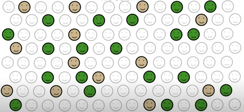
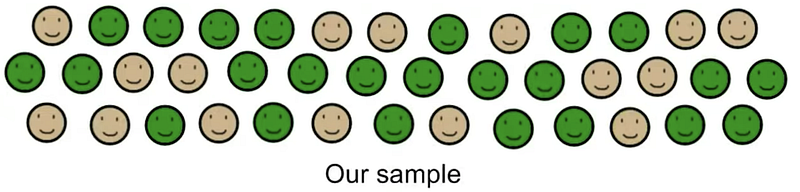
Let’s say we sampled 40 people randomly.

24 out of these 40 answered “tea” while the remaining 16 selected “coffee” i.e 60% selected “tea”.

Now, the question is how confident are we with this guess of 60%. We can’t obviously be 100% sure because we just sampled 40 people from the entire population. So, we give a confidence interval instead.

Confidence Interval (CI) is a range of possible values for an unknown parameter associated with a confidence level of γ that the actual parameter can fall into the suggested range.

In simple words, we want to say that we’re 95 % confident that this value is between x % and y %.

We can’t repeat this exercise multiple times. So, we employ a technique where in we replicate our samples many times i.e

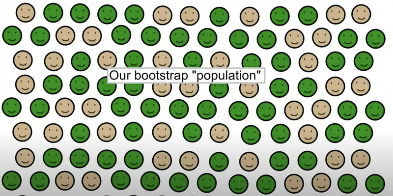
We’ll now take a random sample of the same size (40) from this made up population and let’s say this time we 20 for tea and 20 for coffee. We’ll repeat this process thousands of times.

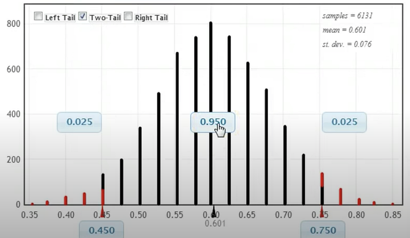
As expected, most of them end up near the original value of 60 but some values lie to the left and some lie to the right. 95% of the times this value was between 45% and 75%.

So, we can say that we are 95% confident that the proportion of Americans that like tea more than coffee is between 45% and 75%.

Check out my related articles:

• Robustness of Modern Deep Learning Systems with a special focus on NLP
• Out-of-Distribution Detection in Deep Neural Networks

References:

1. Xia, Mengzhou, et al. “Predicting performance for natural language processing tasks.” arXiv preprint arXiv:2005.00870 (2020).
2. Ye, Zihuiwen, et al. “Towards More Fine-grained and Reliable NLP Performance Prediction.” arXiv preprint arXiv:2102.05486 (2021).