Summary

The article provides an introduction to the calculus of variations, focusing on the Euler-Lagrange equation and its application in finding the shortest path between two points.

Abstract

The article delves into the mathematical field of calculus of variations, which is explored in the context of an IB Mathematics Internal Assessment. It explains the intuition behind the subject through the classic problem of identifying the shortest path between two points, a challenge that calculus of variations addresses by proving the optimality of a straight line mathematically. The core of the article is the derivation of the Euler-Lagrange equation, a fundamental result in the calculus of variations that is used to find functions that make a functional stationary. The Euler-Lagrange equation is derived by considering an integral that represents a generalized version of the arc length of a path and by using variations of the path to find the stationary value of the integral. The article concludes by applying the Euler-Lagrange equation to confirm that the shortest path between two points is indeed a straight line.

Opinions

The author suggests that the calculus of variations is a natural extension of optimization problems in single variable calculus.
The article implies that the Euler-Lagrange equation is the calculus of variations' equivalent to setting the derivative to zero in single variable calculus for finding stationary points.
The author appears to value the mathematical rigor provided by the Euler-Lagrange equation in proving what may seem intuitively obvious, such as the shortest path between two points being a straight line.
The article conveys that the calculus of variations deals with functionals, which are functions of functions, indicating a level of complexity beyond that of single variable calculus.
By referencing external sources, the author acknowledges the existing body of knowledge in the field and the contributions of other mathematicians to the understanding of the calculus of variations.

Calculus of Variations and the Euler-Lagrange Equation

In this article, I will be introducing a field in mathematics known as calculus of variations which I explored in my IB Mathematics Internal Assessment.

What is Calculus of Variations?

To understand the intuition behind calculus of variations, it may help to consider a simple scenario where it would be used: finding the shortest path between two points. While it is obvious that the answer is a straight line, calculus of variations provides a way of mathematically proving it.

Consider an arbitrary path y(x) that joins the points (x₁, y₁) and (x₂, y₂). Using our knowledge of calculus, it is known that the arc length of this path can be expressed as the following integral:

The arc length of an arbitrary path y(x) from x₁ to x₂

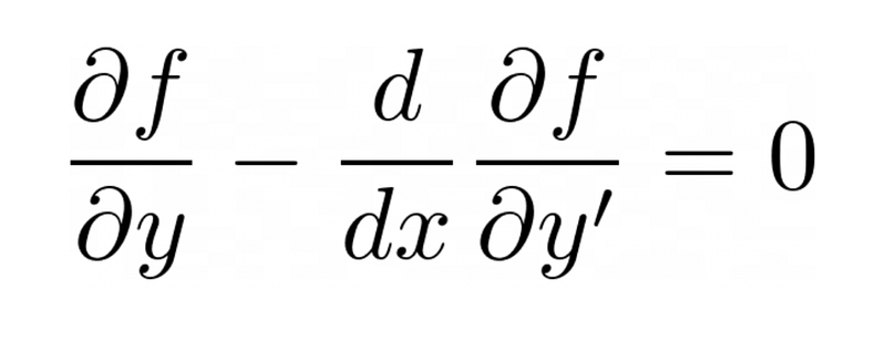
Hence, our goal is to find a function y(x) for which the above integral is a minimum. This is analogous to optimization in single variable calculus where the goal is to find a certain point for which the value of a function is stationary. However, in this case it is much more complicated because now we are attempting to find a certain function for which a functional (a function of functions) is stationary. While in single variable calculus this was simply done by finding the points at which the derivative of the function is equal to zero, a more complex approach must be taken for calculus of variations as a functional is dependent on a function and not a single variable. Instead, an equation known as the Euler-Lagrange equation must be derived.

Deriving the Euler-Lagrange Equation

In order to derive the Euler-Lagrange Equation I will be adapting an already existing derivation.

First, we will consider a generalized version of the above integral that can fit other similar problems:

While in single variable calculus we could differentiate this with respect to a variable, in this case S is dependent on a function and it doesn’t make sense to differentiate something with respect to a function. However, what can be done is the express possible functions for y(x) in terms of a variable.

In order to do this, we first assume that y(x) is the correct path that makes S stationary. Any other curve can be expressed as Y(x) = y(x) + αη(x) where η(x) is any function that satisfies η(x₁) = η(x₂) = 0, and α is a parameter that stretches η(x). The following diagram illustrates this situation:

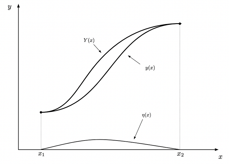
Notice how changing the value of α will stretch η(x) and hence change the shape of Y(x) but the end points will always be fixed, making it a valid curve connecting the two points. Now we can rewrite the expression for S:

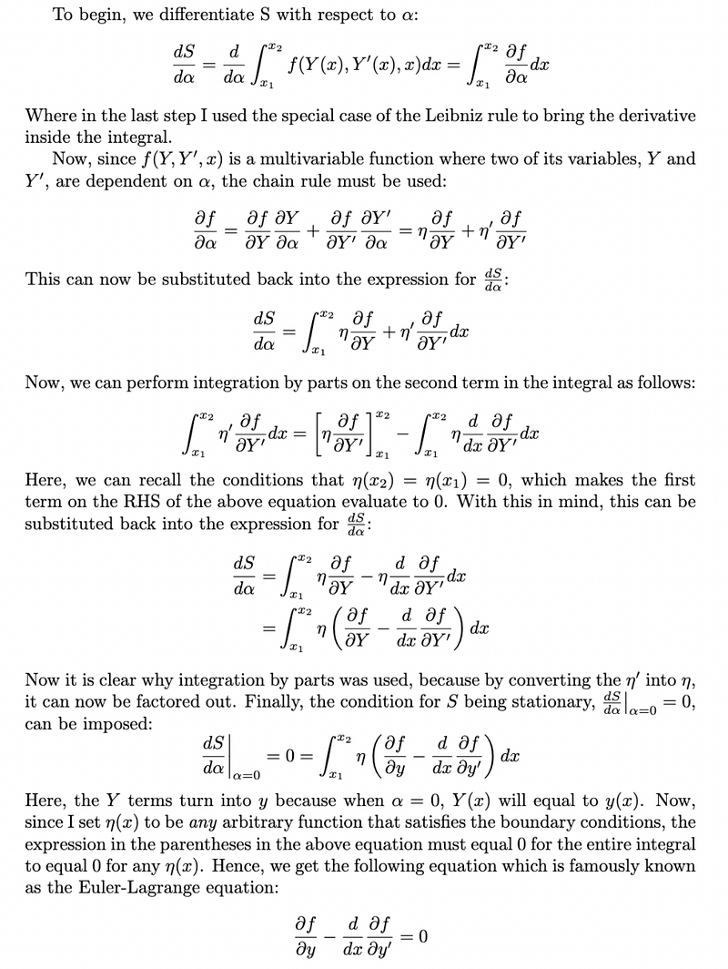
In the above expression, S changes with respect to different values of α, making it a function of α. Recalling from single variable calculus that the stationary value of a function is found when its derivative is equal to 0, the following equation is true:

With this in mind, the following derivation:

The Shortest Path Between Two Points

Equipped with the Euler-Lagrange equation, we can now apply it to the question about the shortest path between two points. Looking back at the expression for the arc length of a curve, the function f in the Euler-Lagrange equation will be the integrand of that expression. Substituting this into the Euler-Lagrange equation and simplifying, we get the following:

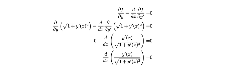
Hence, the expression in the parentheses will be a constant since its derivative is equal to zero. This will give a differential equation that can be solved relatively easily:

Since both c and d are constants, this expression precisely in the form of y=mx+b, proving that the shortest path between two points is indeed a straight line.

References

Calculus II — Arc Length. (2023). Lamar.edu. https://tutorial.math.lamar.edu/classes/calcii/arclength.aspx

‌Taylor, J. R. (2005). Classical mechanics. University Science Books.