
Building a Smart City: An End-to-End Big Data Engineering Project
In today’s fast-paced world, with cities growing quickly and technology advancing at an incredible rate, the idea of smart cities has become a key solution for making urban living more sustainable and efficient. At the heart of smart cities, there’s a big focus on using Big Data, the Internet of Things (IoT), and cloud computing. These technologies are crucial for improving how cities work and making life better for people living in them.
This article takes a close look at a big project that’s all about using these technologies to build a smart city solution from start to finish. We’re talking about using Docker to keep things organized, AWS Cloud for storing and processing data, Apache Spark for handling big chunks of data, and various IoT services to gather data from all over the city. By diving into this project, we’re showing how it’s possible to bring together all these advanced technologies to help cities run smarter. This isn’t just about the tech, though. It’s also about setting an example for how cities can use these tools to tackle real-world problems, making urban areas better places to live.
Introduction
Smart cities are essentially about leveraging the latest in data and technology to significantly enhance various aspects of urban infrastructure and public services, among other areas. The essence of this project lies in its ambitious goal to tap into the vast potential of Big Data. By collecting, processing, and analyzing a wide array of data points from across the city, such as traffic patterns, weather conditions, and emergency incident reports, the project aims to bring about a transformative improvement in urban living.
The idea is not just to gather data for the sake of it but to use this information intelligently. By understanding traffic flows, for instance, we can optimize signal timings and reduce congestion, making commutes faster and less frustrating for everyone. Similarly, by analyzing weather data, cities can better prepare for and respond to adverse conditions, minimizing disruptions and ensuring public safety. And when it comes to emergency incidents, real-time data analysis can help in deploying resources more efficiently, ensuring quicker response times and potentially saving lives.
But the project’s ambitions go beyond just solving these immediate challenges. It’s about creating a framework that allows for continuous improvement and innovation in how cities operate. By establishing a robust data infrastructure, cities can become more adaptive and responsive to the needs of their residents, paving the way for a future where urban environments are not just places where people live but are dynamic, efficient, and sustainable communities that enhance the quality of life for all their inhabitants.
Background of the Project
The project at hand explores the integration of Big Data, the Internet of Things (IoT), and cloud computing to enhance urban mobility, using a case study of a driver’s journey from Central London to Birmingham. This journey, covering approximately 120 miles, serves as an ideal scenario to demonstrate how real-time data collection and analysis can significantly improve the driving experience. By collecting data on vehicle performance, GPS tracking, weather conditions, traffic congestion, and emergency incidents in real-time, the project aims to optimize route selection, reduce travel times, and enhance safety. The utilization of technologies such as Docker for application containerization, AWS Cloud for data storage and processing, and Apache Spark for big data analysis, alongside various IoT services for data collection, underpins this smart city solution.
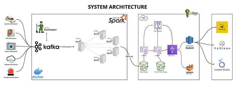
System Architecture
The project’s architecture is designed to be scalable, fault-tolerant, and capable of handling real-time data processing. It integrates Docker containers for deploying services like Zookeeper, Kafka, and Apache Spark in a master-worker architecture. AWS Cloud services are used for storage, data warehousing, and analytics, while IoT services facilitate data collection from various sources.
Containerization and Project Setup
Docker is a platform that enables developers to package applications into containers — standardized executable components combining application source code with the operating system (OS) libraries and dependencies required to run that code in any environment. This means that whether you’re working on your local development machine, in a test environment, or in production, Docker ensures that your application runs exactly the same way by providing a consistent environment. You can learn more about docker here.
Zookeeper:
Zookeeper is a centralized service for maintaining configuration information, naming, providing distributed synchronization, and providing group services. In the context of Kafka, which is a distributed streaming platform, Zookeeper plays a critical role in managing and coordinating Kafka brokers. It helps in leader election for partitions, keeps track of the status of Kafka cluster nodes, and maintains a list of Kafka topics and messages.
zookeeper:
      image: confluentinc/cp-zookeeper:7.4.0
      hostname: zookeeper
      container_name: zookeeper
      ports:
        - "2181:2181"
      environment:
        ZOOKEEPER_CLIENT_PORT: 2181
        ZOOKEEPER_TICK_TIME: 2000
      healthcheck:
        test: ['CMD', 'bash', '-c', "echo 'ruok' | nc localhost 2181"]
        interval: 10s
        timeout: 5s
        retries: 5
      networks:
- datamasterylab- Image: Uses
confluentinc/cp-zookeeper:7.4.0, optimized for Kafka. - Hostname/Container Name: Both set to
zookeeperfor easy identification. - Ports: Exposes port
2181, Zookeeper's default client connection port. - Environment Variables:
ZOOKEEPER_CLIENT_PORT:2181, for client connections.ZOOKEEPER_TICK_TIME:2000ms, the base time unit in Zookeeper.- Healthcheck: Checks Zookeeper’s health by sending
ruokviancto port2181, ensuring it responds withimok. Runs every 10 seconds, with a 5-second timeout and up to 5 retries. - Networks: Joins the
datamasterylabnetwork for intra-service communication.
Kafka Broker:
Kafka is designed for building real-time streaming data pipelines and applications that adapt to the data streams. It can publish, subscribe to, store, and process streams of records in real-time. This makes Kafka a key component in scenarios where you need to process and analyze large volumes of data with minimal latency.
broker:
    image: confluentinc/cp-server:7.4.0
    hostname: broker
    container_name: broker
    depends_on:
      zookeeper:
        condition: service_healthy
    ports:
      - "9092:9092"
      - "9101:9101"
    environment:
      KAFKA_BROKER_ID: 1
      KAFKA_ZOOKEEPER_CONNECT: 'zookeeper:2181'
      KAFKA_LISTENER_SECURITY_PROTOCOL_MAP: PLAINTEXT:PLAINTEXT,PLAINTEXT_HOST:PLAINTEXT
      KAFKA_ADVERTISED_LISTENERS: PLAINTEXT://broker:29092,PLAINTEXT_HOST://localhost:9092
      KAFKA_METRIC_REPORTERS: io.confluent.metrics.reporter.ConfluentMetricsReporter
      KAFKA_OFFSETS_TOPIC_REPLICATION_FACTOR: 1
      KAFKA_GROUP_INITIAL_REBALANCE_DELAY_MS: 0
      KAFKA_CONFLUENT_LICENSE_TOPIC_REPLICATION_FACTOR: 1
      KAFKA_CONFLUENT_BALANCER_TOPIC_REPLICATION_FACTOR: 1
      KAFKA_TRANSACTION_STATE_LOG_MIN_ISR: 1
      KAFKA_TRANSACTION_STATE_LOG_REPLICATION_FACTOR: 1
      KAFKA_JMX_PORT: 9101
      KAFKA_JMX_HOSTNAME: localhost
      KAFKA_CONFLUENT_SCHEMA_REGISTRY_URL: http://schema-registry:8081
      CONFLUENT_METRICS_REPORTER_BOOTSTRAP_SERVERS: broker:29092
      CONFLUENT_METRICS_REPORTER_TOPIC_REPLICAS: 1
      CONFLUENT_METRICS_ENABLE: 'false'
      CONFLUENT_SUPPORT_CUSTOMER_ID: 'anonymous'
    networks:
      - datamasterylab
    healthcheck:
      test: [ "CMD", "bash", "-c", 'nc -z localhost 9092' ]
      interval: 10s
      timeout: 5s
retries: 5- Image: Utilizes
confluentinc/cp-server:7.4.0, tailored for Kafka operations. - Hostname/Container Name: Identified as
brokerfor simplicity and clarity. - Dependency: Waits for
zookeeperto be healthy before starting, ensuring proper order of service startup. - Ports: Opens ports
9092for Kafka client connections and9101for JMX (Java Management Extensions) monitoring. - Environment Variables: Configures Kafka for basic operation, including:
KAFKA_BROKER_ID: Unique identifier for the broker within the cluster.KAFKA_ZOOKEEPER_CONNECT: Connection string for Zookeeper.KAFKA_ADVERTISED_LISTENERS: Addresses that this broker advertises to producers and consumers.KAFKA_METRIC_REPORTERSand related metrics settings: Configured for monitoring, with metrics reporting disabled ('false').- Replication factors set to
1for various internal topics, suitable for development but not for production. KAFKA_JMX_PORT: Port9101for JMX monitoring.- Networks: Connects to the
datamasterylabnetwork for communication with other services like Zookeeper. - Healthcheck: Uses
ncto check the broker's availability on port9092, ensuring the service is ready for connections.
Apache Spark Master-Worker Architecture:
Apache Spark is a unified analytics engine for large-scale data processing. It supports a wide array of tasks, including batch processing, real-time streaming, machine learning, and graph processing. Spark can run in a master-worker architecture, where the master node is responsible for distributing the tasks among worker nodes, which then process the data. The master node manages resource allocation, job scheduling, and communication between the Spark application and the workers.
x-spark-common: &spark-common
  image: bitnami/spark:latest
  volumes:
    - ./jobs:/opt/bitnami/spark/jobs
  command: bin/spark-class org.apache.spark.deploy.worker.Worker spark://spark-master:7077
  depends_on:
    - spark-master
  environment:
    SPARK_MODE: worker
    SPARK_WORKER_CORES: 2
    SPARK_WORKER_MEMORY: 1g
    SPARK_MASTER_URL: spark://spark-master:7077
  networks:
    - datamasterylab
spark-master:
    image: bitnami/spark:latest
    volumes:
      - ./jobs:/opt/bitnami/spark/jobs
    command: bin/spark-class org.apache.spark.deploy.master.Master
    ports:
      - "9090:8080"
      - "7077:7077"
    networks:
- datamasterylab spark-worker-1:
<<: *spark-common spark-worker-2:
<<: *spark-common- spark-master: This service acts as the master node in the Spark cluster. It is responsible for managing the cluster, allocating tasks to worker nodes, and facilitating communication between the Spark application and the worker nodes. The service uses the
bitnami/spark:latestDocker image and exposes ports8080(mapped to9090for access to the Spark UI) and7077for cluster communication. - spark-worker-1 and spark-worker-2: These services serve as the worker nodes in the Spark cluster, executing tasks assigned by the master node. Both workers are configured with the same settings, including 2 CPU cores and 1GB of memory allocated for Spark operations. They also depend on the
spark-masterservice, ensuring the master node is started before the workers. The worker services use the samebitnami/spark:latestimage and are configured to connect to the master node atspark://spark-master:7077. - The
x-spark-commonYAML anchor defines common configurations for the worker nodes, such as the Docker image to use, volume mappings, command to join the cluster as a worker, and environment variables likeSPARK_MODE,SPARK_WORKER_CORES,SPARK_WORKER_MEMORY, andSPARK_MASTER_URL. This approach DRYs (Don't Repeat Yourself) up the configuration, making it easier to maintain and update. - Both the master and worker nodes map a local
./jobsdirectory to/opt/bitnami/spark/jobsinside the containers. This setup allows for easy sharing of Spark jobs and data files between the host and containers.
For folks interested in the video walkthrough, you can follow the coding steps here:
Getting Data From IOT Services
Now that we’ve dealt with the architecture setup, it’s time to bring the services that will be used into limelight.
The IoT devices scattered throughout the city serve as prolific data producers, tirelessly generating a vast array of information on traffic flow, weather conditions, vehicle movements, GPS coordinates, and emergency incidents. This richness of data is absolutely crucial for enabling real-time analytics and informed decision-making, providing city planners, emergency services, and citizens alike with the insights needed to navigate and manage urban life more effectively.
Let’s go ahead and simulate each of the services available for our vehicle heading out Birmingham!
Vehicle Information Generator: This simulate data from vehicles, including speed, location, and health status, to monitor traffic flow and vehicle conditions.
def generate_vehicle_data(device_id):
    location = simulate_vehicle_movement()
    return {
        'id': uuid.uuid4(),
        'deviceId': device_id,
        'timestamp': get_next_time().isoformat(),
        'location': (location['latitude'], location['longitude']),
        'speed': random.uniform(10, 40),
        'direction': 'North-East',
        'make': 'BMW',
        'model': 'C500',
        'year': 2024,
        'fuelType': 'Hybrid'
    }
GPS Information Generator: This aims to provide real-time location data of various entities, aiding in navigation and tracking.
def generate_gps_data(device_id, timestamp, vehicle_type='private'):
    return {
        'id': uuid.uuid4(),
        'deviceId': device_id,
        'timestamp': timestamp,
        'speed': random.uniform(0, 40),  # km/h
        'direction': 'North-East',
        'vehicleType': vehicle_type
    }
Traffic Information Generator: This generates data on traffic density, speed, and incidents to optimize traffic management.
def generate_traffic_camera_data(device_id, timestamp, location, camera_id):
    return {
        'id': uuid.uuid4(),
        'deviceId': device_id,
        'cameraId': camera_id,
        'location': location,
        'timestamp': timestamp,
        'snapshot': 'Base64EncodedString'
    }
Weather Information Generator: Collects data on weather conditions, essential for planning and emergency responses.
def generate_weather_data(device_id, timestamp, location):
    return {
        'id': uuid.uuid4(),
        'deviceId': device_id,
        'location': location,
        'timestamp': timestamp,
        'temperature': random.uniform(-5, 26),
        'weatherCondition': random.choice(['Sunny', 'Cloudy', 'Rain', 'Snow']),
        'precipitation': random.uniform(0, 25),
        'windSpeed': random.uniform(0, 100),
        'humidity': random.randint(0, 100),  # percentage
        'airQualityIndex': random.uniform(0, 500)  # AQL Value goes here
    }
Emergency Incident Generator: Simulates emergency alerts and incidents, enabling quick response and management.
def generate_emergency_incident_data(device_id, timestamp, location):
    return {
        'id': uuid.uuid4(),
        'deviceId': device_id,
        'incidentId': uuid.uuid4(),
        'type': random.choice(['Accident', 'Fire', 'Medical', 'Police', 'None']),
        'timestamp': timestamp,
        'location': location,
        'status': random.choice(['Active', 'Resolved']),
        'description': 'Description of the incident'
    }
Producing IoT Data to Kafka
IoT data producers send the collected data to Kafka, which acts as a central hub for real-time data streams, ensuring efficient data ingestion and processing.
def produce_data_to_kafka(producer, topic, data):
    producer.produce(
        topic,
        key=str(data['id']),
        value=json.dumps(data, default=json_serializer).encode('utf-8'),
        on_delivery=delivery_report
) producer.flush()…and of the data is produced by invoking the function call with the required parameters
produce_data_to_kafka(producer, VEHICLE_TOPIC, vehicle_data)
produce_data_to_kafka(producer, GPS_TOPIC, gps_data)
produce_data_to_kafka(producer, TRAFFIC_TOPIC, traffic_camera_data)
produce_data_to_kafka(producer, WEATHER_TOPIC, weather_data)
produce_data_to_kafka(producer, EMERGENCY_TOPIC, emergency_incident_data)
This gives this output on the kafka broker:
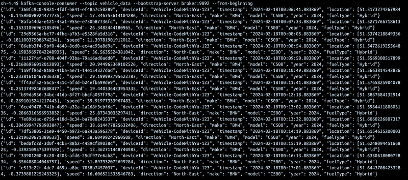
Now that the data has been produced to Kafka, the next thing is to get a realtime consumer waiting for events to drop on the kafka topic to get it triggered and going…
Generating AWS Access Key and Secret Key
Step 1: Access IAM (Identity and Access Management)
- In the AWS Management Console, locate and click on Services.
- Find and select IAM under the Security, Identity, & Compliance category or use the search bar to quickly find IAM.
Step 2: Navigate to Users
- In the IAM dashboard, click on Users in the navigation pane on the left side of the console.
Step 3: Select or Create a New User
For an existing user:
- Click on the username of the user for whom you want to create the access keys.
To create a new user:
- Click on the Add user button.
- Enter the user name.
- Select Programmatic access as the access type. This enables an access key ID and secret access key for the AWS API, CLI, SDK, and other development tools.
- Click Next: Permissions to set permissions for the user. You can add the user to a group with certain policies, copy permissions from an existing user, or attach policies directly.
- Follow through the rest of the steps (Tags, Review) and click Create user at the end.
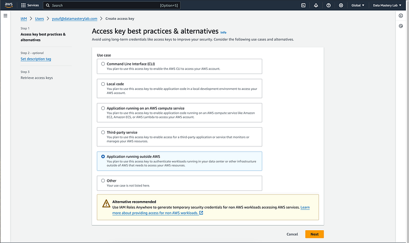
Step 4: Create Access Keys
- If you’re on the user’s summary page (for an existing user):
- Click on the Security credentials tab.
- Scroll down to the Access keys section.
- Click the Create access key button.
Apache Spark Realtime Streaming
The streams of events will be useful to multiple consumers that are listening to events happening on Kafka with Apache Spark. Let’s setup the spark consumer.
spark = SparkSession.builder.appName("SmartCityStreaming") \
  .config("spark.jars.packages",
          "org.apache.spark:spark-sql-kafka-0-10_2.13:3.5.0,"
          "org.apache.hadoop:hadoop-aws:3.3.1,"
          "com.amazonaws:aws-java-sdk:1.11.469") \
  .config("spark.hadoop.fs.s3a.impl", "org.apache.hadoop.fs.s3a.S3AFileSystem") \
  .config("spark.hadoop.fs.s3a.access.key", configuration.get('AWS_ACCESS_KEY')) \
  .config("spark.hadoop.fs.s3a.secret.key", configuration.get('AWS_SECRET_KEY')) \
  .config('spark.hadoop.fs.s3a.aws.credentials.provider',
          'org.apache.hadoop.fs.s3a.SimpleAWSCredentialsProvider') \
  .getOrCreate()
We setup the environment by setting SmartCityStreaming as the appName and bundling a couple of jar packages like sql-kafka, hadoop-aws and aws-java-sdk to our spark streaming app to facilitate the connection between our Kafka cluster and the master-worker architecture setup on Docker.
The structure of the data coming in from the consumer is structured with StructType to give the data a sense of meaning before, during and after consummation.
# vehicle schema
    vehicleSchema = StructType([
        StructField("id", StringType(), True),
        StructField("deviceId", StringType(), True),
        StructField("timestamp", TimestampType(), True),
        StructField("location", StringType(), True),
        StructField("speed", DoubleType(), True),
        StructField("direction", StringType(), True),
        StructField("make", StringType(), True),
        StructField("model", StringType(), True),
        StructField("year", IntegerType(), True),
        StructField("fuelType", StringType(), True),
    ])
# gpsSchema
gpsSchema = StructType([
StructField("id", StringType(), True),
StructField("deviceId", StringType(), True),
StructField("timestamp", TimestampType(), True),
StructField("speed", DoubleType(), True),
StructField("direction", StringType(), True),
StructField("vehicleType", StringType(), True)
]) # trafficSchema
trafficSchema = StructType([
StructField("id", StringType(), True),
StructField("deviceId", StringType(), True),
StructField("cameraId", StringType(), True),
StructField("location", StringType(), True),
StructField("timestamp", TimestampType(), True),
StructField("snapshot", StringType(), True)
]) # weatherSchema
weatherSchema = StructType([
StructField("id", StringType(), True),
StructField("deviceId", StringType(), True),
StructField("location", StringType(), True),
StructField("timestamp", TimestampType(), True),
StructField("temperature", DoubleType(), True),
StructField("weatherCondition", StringType(), True),
StructField("precipitation", DoubleType(), True),
StructField("windSpeed", DoubleType(), True),
StructField("humidity", IntegerType(), True),
StructField("airQualityIndex", DoubleType(), True),
]) # emergencySchema
emergencySchema = StructType([
StructField("id", StringType(), True),
StructField("deviceId", StringType(), True),
StructField("incidentId", StringType(), True),
StructField("type", StringType(), True),
StructField("timestamp", TimestampType(), True),
StructField("location", StringType(), True),
StructField("status", StringType(), True),
StructField("description", StringType(), True),
])The next thing would be to subscribe to Kafka topic and read that till thy kingdom come!
def read_kafka_topic(topic, schema):
    return (spark.readStream
            .format('kafka')
            .option('kafka.bootstrap.servers', 'broker:29092')
            .option('subscribe', topic)
            .option('startingOffsets', 'earliest')
            .load()
            .selectExpr('CAST(value AS STRING)')
            .select(from_json(col('value'), schema).alias('data'))
            .select('data.*')
            .withWatermark('timestamp', '2 minutes')
            )
This functions do just that for us by allowing us to subscribe to any topic and serializing them to the schema we want. To utilize this function we call it as:
vehicleDF = read_kafka_topic('vehicle_data', vehicleSchema).alias('vehicle')
gpsDF = read_kafka_topic('gps_data', gpsSchema).alias('gps')
trafficDF = read_kafka_topic('traffic_data', trafficSchema).alias('traffic')
weatherDF = read_kafka_topic('weather_data', weatherSchema).alias('weather')
emergencyDF = read_kafka_topic('emergency_data', emergencySchema).alias('emergency')
Eventually, we need to write the data to AWS S3 Bucket but we have a challenge here, and that is 5 data streams! We need to be able to write them in parallel to S3 bucket without fail. To achieve this, a function comes in handy:
def streamWriter(input: DataFrame, checkpointFolder, output):
    return (input.writeStream
            .format('parquet')
            .option('checkpointLocation', checkpointFolder)
            .option('path', output)
            .outputMode('append')
            .start())
This function allows us to start each of the streams in parallel and they all run concurrently writing data to S3. In our case, the function is invoked as thus:
query1 = streamWriter(vehicleDF, 's3a://spark-streaming-data/checkpoints/vehicle_data',
             's3a://spark-streaming-data/data/vehicle_data')
query2 = streamWriter(gpsDF, 's3a://spark-streaming-data/checkpoints/gps_data',
             's3a://spark-streaming-data/data/gps_data')
query3 = streamWriter(trafficDF, 's3a://spark-streaming-data/checkpoints/traffic_data',
             's3a://spark-streaming-data/data/traffic_data')
query4 = streamWriter(weatherDF, 's3a://spark-streaming-data/checkpoints/weather_data',
             's3a://spark-streaming-data/data/weather_data')
query5 = streamWriter(emergencyDF, 's3a://spark-streaming-data/checkpoints/emergency_data',
's3a://spark-streaming-data/data/emergency_data')query5.awaitTermination()The awaitTermination function at the end of that blocks sends all the started streams on their journey to heavenly race without interference!
The next thing to do is to submit out spark job to our spark master-worker cluster.
docker exec -it smartcity-spark-master-1 spark-submit \
--master spark://spark-master:7077 \
--packages org.apache.spark:spark-sql-kafka-0-10_2.12:3.5.0,org.apache.hadoop:hadoop-aws:3.3.1,com.amazonaws:aws-java-sdk:1.11.469 \
jobs/spark-city.py
Once submitted, the log looks like this:
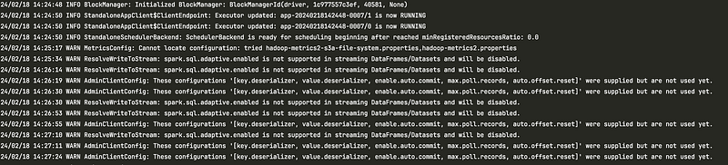
On the UI, we can follow the process to see the progress of submission:

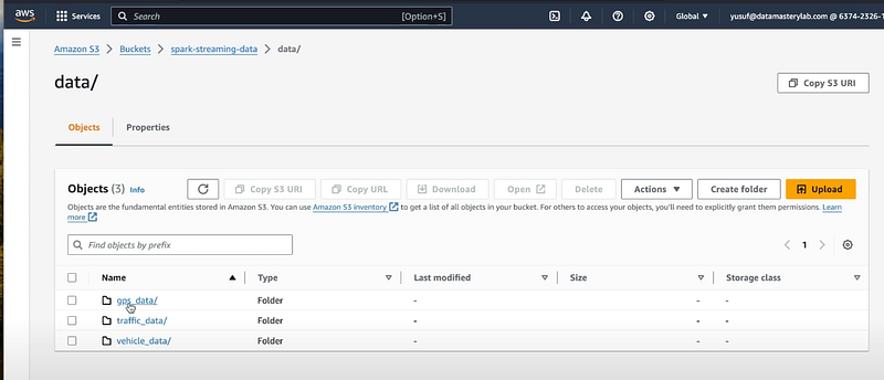
Eventually, in our S3 bucket, we can see the data populated correctly.
Step 1: Creating AWS Glue crawler
- In the AWS Management Console, click on Services to open the services list.
- Find and select Glue under the Analytics category, or use the search bar at the top to search for Glue.
Step 2: Navigate to Crawlers
- In the AWS Glue Console, in the navigation pane on the left side, click on Crawlers under the Data Catalog section.
Step 4: Add a New Crawler
- Click on the Add crawler button to start the process of creating a new crawler.
Step 5: Specify Crawler Info
- Crawler name: Enter a name for your crawler.
- Crawler description (optional): Provide a description for your crawler.
- Tags (optional): Add any tags as needed for organizational purposes.
- Click Next to proceed.
Step 6: Specify Crawler Source Type
- Choose the type of data store. This is typically where your data is stored, such as Amazon S3, JDBC, or DynamoDB.
- For Amazon S3, select the specified path in your bucket where the data resides.
- Click Next to continue.
Step 7: Add a Data Store
- Choose a data store (e.g., Amazon S3).
- Specify the path to your data. For S3, it will be the S3 path to your data files.
- Click Next.
Step 8: Choose an IAM Role
- Select or create an IAM role that AWS Glue can use to access your data sources and targets.
- If you need to create a new role, select Create an IAM role, and give it a name. This role will automatically be granted permissions to access your AWS resources.
- Click Next.
Step 9: Configure Crawler’s Output
- Database: Choose an existing database in the Data Catalog or create a new one where the crawler’s metadata will be stored.
- Prefix added to tables (optional): If you want, specify a prefix for the names of the tables created.
- Configuration options (optional): Configure additional settings as needed, such as adding classifiers, specifying exclusions for S3 paths, or configuring crawler to crawl new folders only.
- Click Next.
Step 10: Review and Finish
- Review all the configurations you’ve made.
- Click Finish to create the crawler.
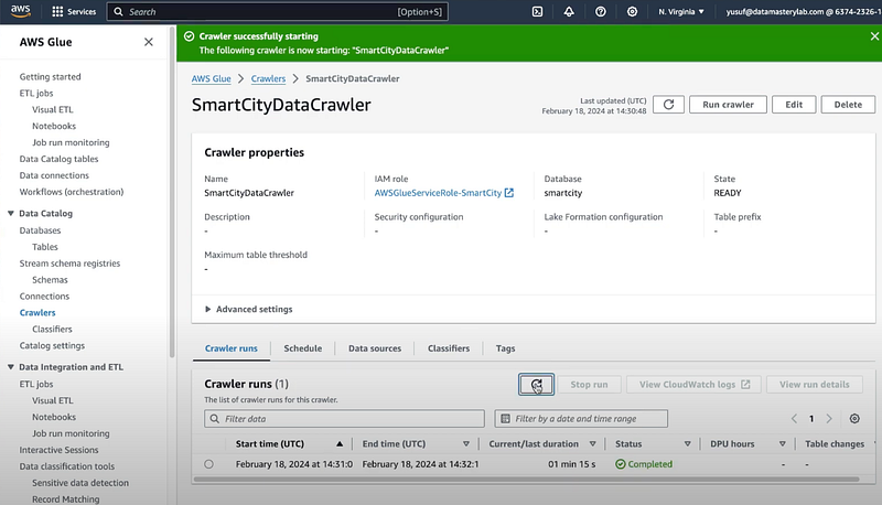
Step 11: Run the Crawler
- After creating the crawler, you’ll be redirected to the crawlers list page.
- Select the checkbox next to your newly created crawler.
- Click on the Run crawler button to start the crawling process.
The crawler will now scan your specified data source, classify the data, and create metadata tables in the AWS Glue Data Catalog. Depending on the size and complexity of your data source, this process may take several minutes to complete.
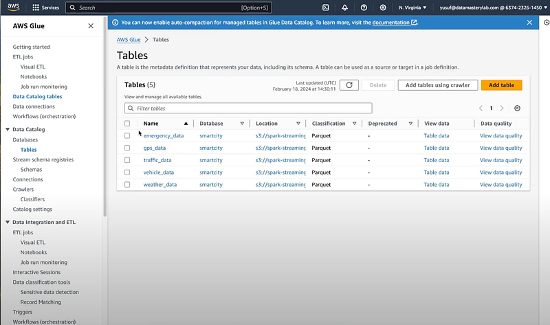
Step 12: Verify the Crawler and Data Catalog
- Once the crawler has finished running, you can navigate to the Tables section in the AWS Glue Console to view the tables and schema it has created.
- You can also check the crawler’s logs for any errors or issues encountered during the run.
You can verify the result of the data crawling by going to AWS Glue -> Tables.
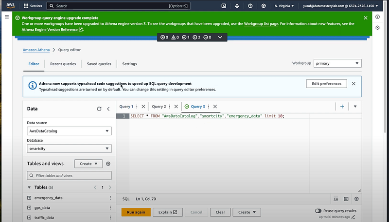
Now, let’s head on to Athena to run sample queries on our data.
Before heading to the final section, consider giving me a follow on all social media platforms, clap and add comments to show support.
- Github: airscholar
- Twitter: @YusufOGaniyu
- LinkedIn: Yusuf Ganiyu
- Youtube: CodeWithYu
Creating Redshift Cluster
Step 1: Open Amazon Redshift Console
- Click on Services in the AWS Management Console.
- Select Redshift under the Database category, or use the search bar at the top to search for Redshift.
Step 2: Launch and Configure Your Redshift Cluster
- In the Redshift Dashboard, click on the Create cluster button.
2. Fill in the necessary details for your cluster configuration:
Cluster details:
- Cluster identifier: Enter a unique name for your cluster.
- Node type: Choose the node type that fits your performance and budget needs. For example,
dc2.largefor general-purpose computing orra3.xlplusfor optimized storage and computing. - Nodes: Specify the number of compute nodes. You can start with 2 nodes for a multi-node setup or choose a single-node cluster for simpler, smaller workloads.
Database configurations:
- Database name: Enter a name for your default database. If you leave this blank, AWS creates a database named
dev. - Database port: The default port is 5439. You can change it if necessary.
- Master username and password: Create a master username and password for your database.
Cluster permissions:
- Available IAM roles: Select an IAM role that Redshift can use to access other AWS services. If you haven’t created a role yet, you can create one by following the prompts.
- Additional configurations: Adjust network and security settings, such as VPC, security groups, and whether the cluster is publicly accessible. For initial setups, the default options might suffice, but ensure the network settings align with your access needs.
Review and launch:
- Review your settings. You can click on Edit in each section to make changes.
- Once satisfied, click on the Create cluster button.
Step 3: Connect to Your Cluster
- Once the cluster status is Available, you can connect to it.
- Navigate to the Clusters page and select your cluster to view its details.
- Note the cluster’s endpoint and JDBC URL, which are needed to connect to your cluster using tools like DBeaver.
Connecting and Querying Redshift Cluster with DBeaver
Once DBeaver is opened, create a new cluster and input the JDBC URL, and the username and password as below:

Connecting AWS Glue to Redshift Cluster
In a new SQL script on DBeaver, let’s import the data catalog from glue into our redshift cluster.
create external schema dev_smartcity
from data catalog
database smartcity
iam_role 'arn:aws:iam::102123451450:role/smart-city-redshift-s3-role'
region 'us-east-1';
Explanation:
- CREATE EXTERNAL SCHEMA dev_smartcity: This line starts the command to create a new external schema named
dev_smartcityin your Redshift cluster. An external schema is a schema that references external data stored in S3, managed by AWS Glue Data Catalog, or another supported service, allowing you to query data stored outside of Redshift. - FROM DATA CATALOG: Specifies that the external schema will be created from the AWS Glue Data Catalog. AWS Glue Data Catalog is a managed service that lets you store, annotate, and share metadata across AWS services.
- DATABASE
smartcity: Identifies the name of the database in the AWS Glue Data Catalog that this external schema will access. In this case, it’ssmartcity. - IAM_ROLE
arn:aws:iam::102123451450:role/smart-city-redshift-s3-role: Specifies the IAM role that Redshift should assume when accessing the external data. This role needs to have the necessary permissions to access the AWS Glue Data Catalog and any underlying data stores (like Amazon S3 buckets) that the catalog references. - REGION
us-east-1: Indicates the AWS region where the AWS Glue Data Catalog database is located. It’s important that this matches the region of the Glue database to ensure connectivity.
You can then easily query data directly using:
select * from dev_smartcity.gps_data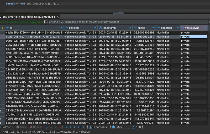
The rest is to connect a visualisation layer like PowerBI, Tableau or Looker studio and start building those beautiful dashboards!
And that’s a wrap!
If you are interested in any of the topics below:
- Python
- Data Engineering
- Data Analytics
- Data Science
- SQL
- Cloud Platforms (AWS/GCP/Azure)
- Machine Learning
- Artificial Intelligence
Like and Follow me on all platforms:
- Github: airscholar
- Twitter: @YusufOGaniyu
- LinkedIn: Yusuf Ganiyu
- Youtube: CodeWithYu
- Medium: Yusuf Ganiyu
I regularly share daily contents on Linkedin, X, Medium & YouTube.
More courses available on datamasterylab.com
You can buy me a coffee:


