Building a Robust Data Pipeline on Databricks using the Lambda Architecture With Sports Data(DIM)

Our last Databricks project introduced us to new concepts using the Medallion architecture to achieve this. In this project, we will dive deeper into Databricks with the Lambda architecture. Finding the right data for a specific project can be challenging. It is often easier to design a project around the available data rather than trying to force data to fit predefined tools or requirements. However, in this project, we will focus on identifying and selecting the most suitable data for the task at hand.

Link to Github Repo at bottom of the page.

First, what is the Lambda Architecture?

Lambda Architecture is a data processing architecture designed to handle massive quantities of data by utilizing both batch and real-time processing methods. The architecture is designed to balance the trade-offs between latency, throughput, and fault tolerance, ensuring high scalability and resilience in big data systems.

Latency: Latency refers to the amount of time it takes for the system to process data and deliver results. Low latency is crucial when real-time or near-real-time data processing is required, such as in financial trading systems, monitoring dashboards, or recommendation engines. The speed layer in Lambda is designed to minimize latency by processing data in real time, so you can get quick but likely less accurate results. The batch layer provides more accurate results but with higher latency because it processes data in larger, less frequent batches.

Throughput: Throughput refers to the amount of data a system can process over a given period of time. High throughput is essential in big data systems because they often need to handle massive volumes of data in a short time. Systems must process vast amounts of data efficiently to keep up with demand. The batch layer handles the bulk of data processing and is optimized for high throughput. It processes large amounts of historical data at once. Meanwhile, the speed layer focuses on processing small, recent data quickly but not necessarily at the same volume as the batch layer.

Fault Tolerance: Fault tolerance refers to the system’s ability to continue functioning correctly even when parts of it fail or encounter errors. In big data systems, where large distributed systems are involved, hardware or software failures are common. Fault tolerance ensures the system can recover from these failures without losing data or significant downtime. The batch layer provides a safety net because even if real-time processing in the speed layer fails, the batch layer will eventually process the data and provide accurate results. This dual-layer system adds fault tolerance to the architecture.

Ensuring High Scalability and Resilience: Scalability refers to the system’s ability to handle increasing amounts of data or requests by adding more resources (such as servers). Lambda Architecture achieves high scalability by splitting the workload between batch and speed layers. The batch layer can scale horizontally (add more nodes to process data in parallel), while the speed layer focuses on handling real-time data efficiently. Resilience means the system can adapt to and recover from disruptions (such as hardware failures, traffic spikes, or unexpected data volumes). Lambda Architecture’s fault tolerance (with separate batch and speed layers) and scalable design make it resilient. Even if one layer fails or slows down, the other layer can continue providing insights, ensuring continuous operation.

Key Components of Lambda Architecture:

Batch Layer

Purpose: The batch layer handles large-scale data that needs to be processed periodically.
Data Store: The raw, immutable data is stored in a distributed file system, like HDFS (Hadoop Distributed File System).
Processing: It performs time-consuming computations (often using tools like Apache Hadoop or Spark) and computes the batch views (aggregated results) that provide accurate but delayed results.
Output: The output of this layer is stored in batch views or precomputed results that are served when needed.

2. Speed Layer (Real-Time Layer)

Purpose: The speed layer processes data in real-time to provide low-latency updates and near-instant results.
Data Store: This layer processes only the recent data that hasn’t yet been processed by the batch layer.
Processing: Tools like Apache Storm, Apache Kafka, or Apache Flink are used for real-time data streaming and analysis.
Output: This layer generates real-time views, which are not as accurate as batch views but provide fresh, up-to-date insights.

3. Serving Layer

Purpose: This layer merges the results from both the batch and speed layers and serves them to applications or users.
Data Store: It stores precomputed results from the batch and speed layers in a way that allows for fast querying, using databases like Cassandra or HBase.
Function: The results from both the batch and real-time views are combined to provide accurate and up-to-date data.

Pros of Lambda Architecture:

Scalability: Can handle massive amounts of data by separating batch and real-time processing.
Fault Tolerance: The batch layer ensures that historical data is processed accurately, even if real-time computations fail.
Flexibility: It allows for both historical and real-time data analysis.

Cons of Lambda Architecture:

Complexity: Maintaining two separate processing pipelines (batch and real-time) increases system complexity.
Maintenance: Managing different code bases for batch and real-time processing can be difficult.

PROJECT OUTLINE;

Now it’s time to start our project.

Steps in the Batch layer;

Understand the data and what we’re trying to accomplish.
Build a scrape script to get the necessary NCAA football data from Ourlads.com and player stats from ESPN.
Using Great Expectations or custom Python scripts, implement data quality checks.
Provision your Databricks Workspace and a Data lake storage resources on Azure.
Set up the environments to enable Selenium to run on Databricks.
Ensure all data quality checks pass before saving DataFrames as Parquet to DBFS.
Save them in your Blob storage container in a new folder named after the current date.
Schedule and automate script to run weekly.

Steps in the Stream layer;

Develop a real-time streaming script that fetches live match data from the ESPN API and stores it efficiently in a Databricks SQL table.
Develop a Databricks dashboard to visualize live match data in real-time. (OPTIONAL)

Steps in the Serving layer;

Provision a PostgreSQL database on Azure Portal.
Design and implement a normalized database schema.
Migrate the relevant data into the PostgreSQL database.

BATCH LAYER

Understand the data and what we’re trying to accomplish.

Overview of NCAA College Football Data

NCAA college football data captures a rich history of the sport, offering detailed insights into player statistics, team performance, game outcomes, and much more. This data has become critical for a variety of purposes, including fan engagement, sports betting, media analysis, and advanced analytics. Here’s an in-depth look into the data types, history, and relevance of NCAA football data from a data engineering perspective.

A Brief History of NCAA Football and Its Data

The National Collegiate Athletic Association (NCAA) was founded in 1906 and has overseen college football since then, organizing thousands of teams and games across the United States. College football has grown into a massive sport, rivaling professional football in terms of viewership, and is an integral part of American sports culture.

Initially, data collection in NCAA football was very limited, focusing mainly on scores, win-loss records, and championship results. However, with the advent of digital technology, the amount and complexity of data have dramatically increased. Modern college football data now includes everything from in-game player statistics to advanced performance metrics like yards per attempt, quarterback efficiency, turnover rates, and even real-time tracking data.

With the explosion of the internet and the availability of APIs, college football data became widely accessible for fans, analysts, teams, and even bettors. Today, platforms like ESPN, Ourlads, and the NCAA’s resources provide comprehensive and live data, laying the groundwork for a wide range of applications, from data analysis to machine learning.

When scraping roster and depth chart data from Ourlads.com and player stats from ESPN for NCAA college football, you’ll be extracting two key datasets:

1. Roster and Depth Chart Data (Ourlads.com):

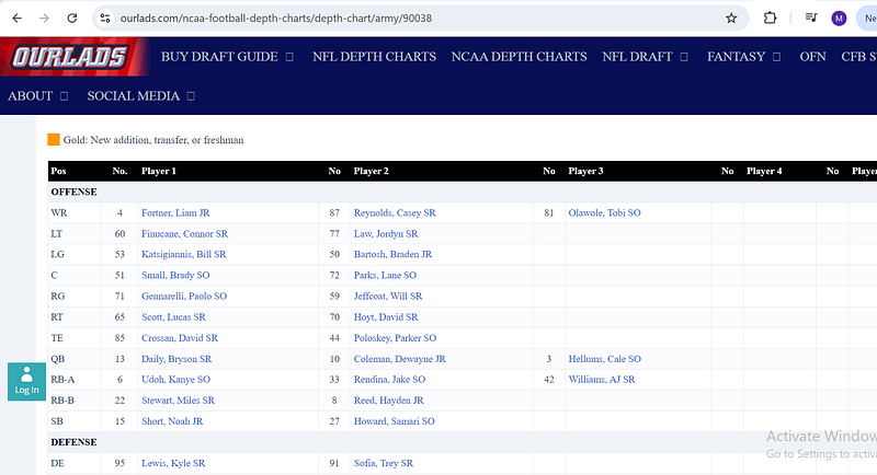
Roster Data: Provides detailed information on players for each team, such as:
Player Name
Position
Jersey Number
Height, Weight, and Age
Year in School (Freshman, Sophomore, etc.)
Depth Chart Data: This shows the current hierarchy of players for each position (starter, backup, third string), which helps in understanding team dynamics and positional strength.

2. Player Stats (ESPN):

ESPN offers detailed player statistics such as:
Passing, Rushing, and Receiving Stats
Tackles, Sacks, and Defensive Plays
Season Totals and Game-by-Game Breakdowns
Advanced Metrics like QB rating, rushing yards per carry, etc.

Build a scrape script to get the necessary NCAA football data from Ourlads.com and player stats from ESPN.

We are going to write 3 scripts;

Two to scrape data from each roster and depth chart link in https://www.ourlads.com/ncaa-football-depth-charts/
Another is to scrape player stats data from ESPN’s https://www.espn.com/college-football/stats/player

The full code will be in the GitHub repo at the end of this article. You don’t need to worry about this code, the major code is the one that will run on Databricks.

import requests  # Library for making HTTP requests
from bs4 import BeautifulSoup  # Library for parsing HTML and XML documents
from fake_useragent import UserAgent  # Generates random User-Agent strings to mimic real browsers
import pandas as pd  # Library for data manipulation and analysis
import great_expectations as ge  # Library for data validation and quality checks

# Set the URL of the NCAA football depth charts page
url = 'https://www.ourlads.com/ncaa-football-depth-charts'

ua = UserAgent()  # Instantiate UserAgent to generate random user agents
userAgent = ua.random  # Generate a random user agent
headers = {'User-Agent': userAgent}  # Set headers with the random User-Agent to avoid bot detection
page = requests.get(url, headers=headers)  # Send an HTTP GET request to the URL
soup = BeautifulSoup(page.content, "html.parser")  # Parse the HTML content of the page with BeautifulSoup

# Find all the team links on the page for scraping depth chart and roster data
team_links = []  # List to store the depth chart URLs for each team
team_link = soup.find_all('div', class_="nfl-dc-mm-team-links")  # Find the divs containing team links
for i in team_link:
    team_links.append('https://www.ourlads.com/ncaa-football-depth-charts/' + i.a['href'])  # Append full URLs for each team

team_links_depth_chart = team_links[1:]  # Store team links for depth charts (skip the first one)

# Create roster URLs by replacing 'depth-chart.aspx' with 'roster.aspx' in the URLs
team_links_roster = [url.replace('depth-chart.aspx', 'roster.aspx') for url in team_links]
team_links_roster = team_links_roster[1:]  # Exclude the first one again

master_df = []  # List to hold DataFrames for each team depth chart

# Function to scrape depth chart data for each team
def get_all_csv(url):
    ua = UserAgent()  # Generate a random User-Agent
    userAgent = ua.random  # Get a random User-Agent string
    head = {'User-Agent': userAgent}  # Set headers for the request
    page = requests.get(url, headers=head)  # Make the GET request to the team URL
    soup = BeautifulSoup(page.content, "html.parser")  # Parse the HTML content

    team_name = soup.find('div', {'class': 'pt-team'}).text.strip()  # Extract the team name from the page

    # Find the table containing the depth chart data
    table = soup.find('table', class_='table table-bordered')  
    headers = [th.text.strip() for th in table.find_all('th')]  # Extract table headers
    rows = []  # List to store all rows of data
    for tr in table.find('tbody').find_all('tr'):  # Iterate through each row in the table body
        cells = [td.text.strip() for td in tr.find_all('td')]  # Extract text from each cell in the row
        rows.append(cells)  # Add the row data to the list

    df = pd.DataFrame(rows, columns=headers)  # Create a DataFrame with the extracted table data
    df['team_name'] = team_name  # Add a new column for the team name
    print(team_name)  # Print the team name (for logging purposes)

    # Fill the 'field_pos' column to classify players into Offense, Defense, or Special Teams
    df['field_pos'] = df['Pos'].where(df['Pos'].isin(['Offense', 'Defense', 'Special Teams']))
    df['field_pos'] = df['field_pos'].ffill()  # Forward fill missing values in 'field_pos'
    
    # Remove rows with these position labels as they are headers, not player data
    df = df[~df['Pos'].isin(['Offense', 'Defense', 'Special Teams', 'OFF', 'ST', 'DEF'])]

    # Rename columns for player positions and string order
    df.rename(columns={'Player 1': '1st String', 'Player 2': '2nd String', 'Player 3': '3rd String', 
                       'Player 4': '4th String', 'Player 5': '5th String', 'Pos': 'Position', 'No.': 'No1'}, inplace=True)

    no_counter = 2  # Initialize counter for other player numbers (No2, No3, etc.)
    new_columns = []  # List to store new column names
    for col in df.columns:  # Loop through columns and rename 'No' columns with sequential numbers
        if col == 'No':
            new_columns.append(f'No{no_counter}')  # Append numbered No columns
            no_counter += 1  # Increment the counter
        else:
            new_columns.append(col)  # Keep other column names unchanged

    df.columns = new_columns  # Update the DataFrame with new column names

    # Concatenate player number and name columns into the first, second, etc., string positions
    df['1st String'] = df['No1'].astype(str) + ' ' + df['1st String']
    df['2nd String'] = df['No2'].astype(str) + ' ' + df['2nd String']
    df['3rd String'] = df['No3'].astype(str) + ' ' + df['3rd String']
    df['4th String'] = df['No4'].astype(str) + ' ' + df['4th String']
    df['5th String'] = df['No5'].astype(str) + ' ' + df['5th String']

    df = df.drop(columns=['No1', 'No2', 'No3', 'No4', 'No5'])  # Drop the redundant number columns

    # Reshape the DataFrame from wide to long format for better structure
    df = df.melt(id_vars=['Position', 'field_pos', 'team_name'], 
                 value_vars=['1st String', '2nd String', '3rd String', '4th String', '5th String'], 
                 var_name='String Order', value_name='Player Name')

    # Extract the player number from the player name
    df['Player Number'] = df['Player Name'].str.extract(r'^(\d+)')
    
    # Remove the player number from the player name field
    df['Player'] = df['Player Name'].str.replace(r'^\d+\s+', '', regex=True)

    # Split the player name into first name and other names
    df[['First Name', 'Other Names']] = df['Player'].str.split(' ', n=1, expand=True)

    # Drop the original 'Player' and 'Player Name' columns
    df = df.drop(columns=['Player Name', 'Player'])

    # Clean up first names and extract the last name and school year
    df['First Name'] = df['First Name'].str.replace(',', '')
    df[['Last Name', 'School year']] = df['Other Names'].str.split(' ', n=1, expand=True)

    df = df.drop(columns=['Other Names'])  # Drop the 'Other Names' column after splitting

    master_df.append(df)  # Append the cleaned DataFrame to the master list

# Loop through each team link to scrape and process depth chart data
for i in team_links_depth_chart:
    get_all_csv(i)

# Combine all the individual team DataFrames into one DataFrame
df_res = pd.concat(master_df)

# Convert the DataFrame to a Great Expectations DataFrame for validation
ge_df = ge.from_pandas(df_res)

# Validate that 'Position' is not null
ge_df.expect_column_values_to_not_be_null('Position')

# Validate that 'field_pos' is not null
ge_df.expect_column_values_to_not_be_null('field_pos')

# Validate that 'team_name' is not null
ge_df.expect_column_values_to_not_be_null('team_name')

# Ensure 'Player Number' contains only numeric values
ge_df.expect_column_values_to_match_regex('Player Number', r'^\d+$')

# Ensure 'String Order' is one of the predefined values
ge_df.expect_column_values_to_be_in_set('String Order', ['1st String', '2nd String', '3rd String', '4th String', '5th String'])

# Ensure 'field_pos' contains only valid values
ge_df.expect_column_values_to_be_in_set('field_pos', ['Defense', 'Offense', 'Special Teams'])

# Run the validations and return the results
results = ge_df.validate()

# Print validation results
results

# If the validation is successful, save the cleaned DataFrame to a CSV file
if results['success']:
    df_res.to_csv('/workspace/sales/sports/college_football_depth_chart.csv', index=False)
else:
    print("Data quality validation failed.")  # Print an error message if validation fails

Depth chart and Roster script with data quality checks using Great Expectations.

This code performs web scraping to extract the NCAA college football depth chart and roster data from the Ourlads website. It uses libraries like requests, BeautifulSoup, and pandas for the scraping and transformation process, and Great Expectations for data quality checks and validation.

Here’s a breakdown of the code:

1. Imports:

requests: For making HTTP requests to the website.
BeautifulSoup (from bs4): To parse and navigate HTML content.
UserAgent (from fake_useragent): To generate a random user agent, mimicking a real browser to avoid bot detection.
pandas: For storing and manipulating scraped data in tabular form (DataFrames).
great_expectations: For validating and ensuring the quality of the data.

2. Web Scraping Setup:

The code begins by setting up the URL for NCAA football depth charts on Ourlads.com.
It creates a random User-Agent to avoid detection by scraping protections.
The content of the webpage is retrieved using requests.get, and parsed with BeautifulSoup to extract specific sections of the page.

3. Scraping Team Links:

soup.find_all locates specific divs containing team links.
These links are stored in the team_links_depth_chart list for future requests.
The roster URLs are created by modifying the depth chart URLs.

4. Scraping and Processing Depth Chart Data (get_all_csv function):

This function scrapes individual team depth chart data from each team’s page.
It processes an HTML table containing player information (positions, string order, etc.) and converts it into a pandas DataFrame.
The table’s structure is cleaned by renaming columns, extracting and formatting player names, and organizing the data by positions like “Offense”, “Defense”, or “Special Teams”.
The resulting DataFrame is appended to a master_df list for all teams.

5. Data Validation with Great Expectations:

The concatenated data is converted into a Great Expectations DataFrame for validation.
A series of data expectations are defined:
Ensuring that columns like Position, field_pos, and team_name are not null.
Ensuring that Player Number contains only numeric values.
Validating that String Order and field_pos contain specific expected values.
After validation, if the data passes the checks, it is saved to a CSV file.

6. Scraping Roster Data (get_roster function):

Similar to the depth chart scraper, this function extracts and processes player roster information from each team’s roster page.
It cleans and formats the player names, player numbers, positions, height, and weight.
The formatted height and weight are converted into a readable format for consistency.

7. Roster Data Validation:

Similar expectations are defined for the roster data:
Ensuring Player Number is not null and is an integer.
Validating that Weight is between 100 and 450 pounds.
Checking that team_name and Position are not null.
If the validation passes, the data is saved to a CSV file.

8. Final Steps:

If both depth chart and roster data pass the validation, the results are saved to CSV files for further use.

The next script gets the player's stats;

from selenium.webdriver import Chrome  # Import Chrome WebDriver to control the browser
from selenium.webdriver.support.ui import Select  # For interacting with dropdown elements
from selenium.webdriver.support.ui import WebDriverWait  # For waiting until certain conditions are met
from selenium.webdriver.common.by import By  # For locating elements by various attributes (e.g., ID, ClassName)
from selenium import webdriver  # For handling web browser interactions
from selenium.webdriver.chrome.options import Options  # For customizing Chrome browser options
from selenium.webdriver.support import expected_conditions as EC  # For conditions to wait on, like element to be clickable
from fake_useragent import UserAgent  # For generating random user-agent strings to simulate different browsers
from selenium.webdriver.chrome.service import Service  # To start the Chrome driver service
import time  # For adding delays to control script execution
import requests  # For making HTTP requests
from bs4 import BeautifulSoup  # For parsing HTML content
import pandas as pd  # For manipulating data and creating DataFrames
import re  # For regular expressions (used for pattern matching)

# URLs to scrape data from ESPN's college football player stats pages
urls = ('https://www.espn.com/college-football/stats/player',
        'https://www.espn.com/college-football/stats/player/_/stat/rushing',
        'https://www.espn.com/college-football/stats/player/_/stat/receiving',
        'https://www.espn.com/college-football/stats/player/_/view/defense',
        'https://www.espn.com/college-football/stats/player/_/view/scoring')

# Function to scrape data from each URL
def get_all_stats(url):
    # Path to ChromeDriver executable (adjust as per your local setup)
    service = Service(executable_path=r'chromedriver-win64\chromedriver-win64\chromedriver.exe')
    
    options = Options()  # Create Chrome browser options object
    ua = UserAgent()  # Instantiate UserAgent to generate random user agents
    userAgent = ua.random  # Generate a random user-agent string
    options.add_argument(f'user-agent={userAgent}')  # Set the random user-agent string in browser options
    options.add_argument('--blink-settings=imagesEnabled=false')  # Disable loading images to speed up page load
    
    # Initialize the Chrome WebDriver with the service and options
    driver = webdriver.Chrome(service=service, options=options)
    driver.get(url)  # Load the specified URL in the Chrome browser
    
    time.sleep(5)  # Pause for 5 seconds to allow the page to load completely
    
    # Continuously click the "Show More" button until no more data can be loaded
    while True:
        try:
            # Locate the "Show More" button by its class name
            element = driver.find_element(By.CLASS_NAME, 'AnchorLink.loadMore__link')
            # Wait until the "Show More" button is clickable
            WebDriverWait(driver, 20).until(EC.element_to_be_clickable((By.CLASS_NAME, 'AnchorLink.loadMore__link')))
            # Scroll the "Show More" button into view
            driver.execute_script("arguments[0].scrollIntoView();", element)
            # Click the "Show More" button to load more data
            driver.execute_script("arguments[0].click();", element)
            time.sleep(5)  # Pause for 5 seconds between clicks
        except Exception as e:  # Catch any exception if "Show More" button is not found
            print(e)  # Print the exception message
            break  # Exit the loop if no more data can be loaded
        print("Complete")  # Log progress when a "Show More" click is successful
    
    print('all show more clicked')  # Indicate that all data has been loaded
    
    page = driver.page_source  # Get the page source (HTML content)
    
    # Clean the HTML by removing unwanted rows (optional step)
    cleaned_html = re.sub(r'<tr class="Table__TR.Table__even">.*?</tr>', '', str(page), flags=re.DOTALL)
    
    # Parse the cleaned HTML content using BeautifulSoup
    soup = BeautifulSoup(cleaned_html, 'html.parser')
    
    tables = soup.find_all('table')  # Find all table elements in the HTML
    driver.quit()  # Close the Chrome browser
    
    dataframes = []  # List to store extracted data as DataFrames
    
    # Loop over each table found in the HTML and extract it into a pandas DataFrame
    for table in tables:
        headers = [th.text.strip() for th in table.find_all('th', class_='Table__TH')]  # Extract table headers
        headers = list(filter(None, headers))  # Filter out empty headers
        
        rows = []  # List to store rows of table data
        # Extract data from each row in the table
        for row in table.find_all('tr'):
            cells = [cell.text.strip() for cell in row.find_all('td')]  # Extract text from each table cell
            if cells:  # Avoid adding empty rows
                rows.append(cells)
        
        # Create a DataFrame if headers exist; otherwise, use default row indexing
        if headers:
            df = pd.DataFrame(rows, columns=headers)  # Create DataFrame with headers
        else:
            df = pd.DataFrame(rows)  # Create DataFrame without headers
        
        dataframes.append(df)  # Append the DataFrame to the list
    
    # Concatenate all the DataFrames for the current page into a single DataFrame
    dataframes = pd.concat(dataframes, axis=1)
    
    # Extract the team abbreviation from the 'Name' column
    dataframes['Team'] = dataframes['Name'].str.extract(r'([A-Z]{2,})$')
    
    # Remove the uppercase letters (team abbreviations) from the 'Name' column
    dataframes['Name'] = dataframes['Name'].str.replace(r'([A-Z]{2,})$', '', regex=True).str.strip()
    
    # Save the DataFrame to a CSV file using part of the URL as the filename
    dataframes.to_csv(f"{url.rstrip('/').split('/')[-1]}.csv")

# Loop through the list of URLs and scrape data from each URL
for i in urls:
    get_all_stats(i)  # Call the function to scrape and process data for each URL

Imports: Required libraries for web scraping (selenium, bs4, pandas, etc.) are imported.

URLs: A tuple containing different ESPN URLs for scraping football stats.

Function (get_all_stats):

Webdriver Initialization: Uses Chrome WebDriver with a random user-agent and disabled images to speed up loading.
Show More Handling: The script keeps clicking the “Show More” button until all content is loaded.
Page Parsing: The content of the page is retrieved and parsed using BeautifulSoup, and unwanted rows are removed using regex.
Table Extraction: Extracts tables from the page, creates DataFrames, and cleans the data (removing team abbreviations from player names).
Saving Data: The resulting DataFrame is saved as a CSV file.

Loop Over URLs: For each URL in the urls tuple, the script scrapes and processes the data by calling get_all_stats.

NOTE: For the second script, you’ll need to write your own data quality checks.

Provision your Databricks Workspace and a Data lake storage resources on Azure.

This part is quite straightforward if you’ve been following the other Databricks tutorials, even if you haven’t, it’s still quite simple and a little challenge for you will help you grow faster.

Set up the environments to enable Selenium to run on Databricks.

After provisioning Databricks, create a new notebook and a personal compute cluster for the sake of this project. Once your notebook is successfully attached to your cluster, paste this.

dbutils.fs.mkdirs("dbfs:/databricks/scripts/")
dbutils.fs.put("/databricks/scripts/selenium-install.sh","""
#!/bin/bash
%sh
LAST_VERSION="https://www.googleapis.com/download/storage/v1/b/chromium-browser-snapshots/o/Linux_x64%2FLAST_CHANGE?alt=media"
VERSION=$(curl -s -S $LAST_VERSION)
if [ -d $VERSION ] ; then
  echo "version already installed"
  exit
fi
 
rm -rf /tmp/chrome/$VERSION
mkdir -p /tmp/chrome/$VERSION
 
URL="https://www.googleapis.com/download/storage/v1/b/chromium-browser-snapshots/o/Linux_x64%2F$VERSION%2Fchrome-linux.zip?alt=media"
ZIP="${VERSION}-chrome-linux.zip"
 
curl -# $URL > /tmp/chrome/$ZIP
unzip /tmp/chrome/$ZIP -d /tmp/chrome/$VERSION
 
URL="https://www.googleapis.com/download/storage/v1/b/chromium-browser-snapshots/o/Linux_x64%2F$VERSION%2Fchromedriver_linux64.zip?alt=media"
ZIP="${VERSION}-chromedriver_linux64.zip"
 
curl -# $URL > /tmp/chrome/$ZIP
unzip /tmp/chrome/$ZIP -d /tmp/chrome/$VERSION
 
mkdir -p /tmp/chrome/chrome-user-data-dir
 
rm -f /tmp/chrome/latest
ln -s /tmp/chrome/$VERSION /tmp/chrome/latest
 
# to avoid errors about missing libraries
sudo apt-get update
sudo apt-get install -y libgbm-dev
""", True)
display(dbutils.fs.ls("dbfs:/databricks/scripts/"))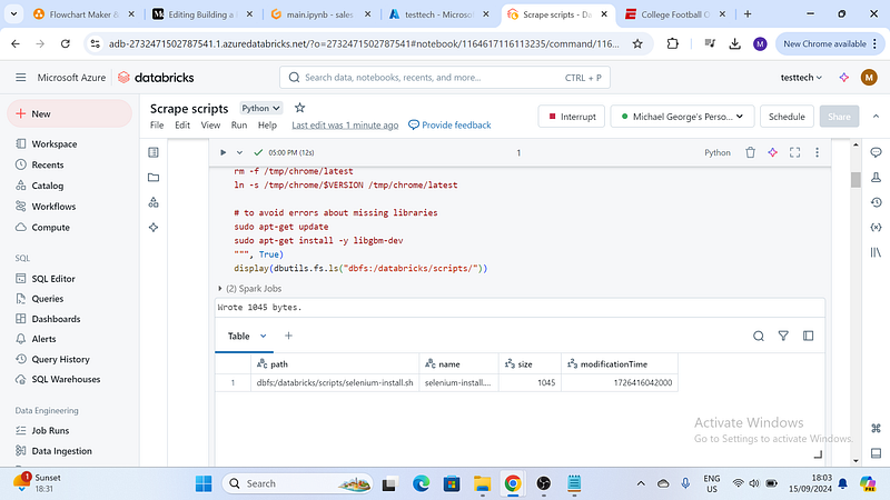

Directory Creation: It creates a folder dbfs:/databricks/scripts/ in Databricks' file system.

Shell Script: It writes a shell script (selenium-install.sh) that automates the download and installation of the latest Chromium browser and Chromedriver from Google's storage. It includes updating the system and installing any missing dependencies (libgbm-dev).

File Verification: The last line lists the files in the /databricks/scripts/ directory to ensure the shell script was created.

Next, type this and run all cells.

%sh
/dbfs/databricks/scripts/selenium-install.sh

After a successful code run our selenium code was slightly changed to work on Databricks. Remember to pip install selenium.

from selenium import webdriver
from selenium.webdriver.chrome.service import Service
from fake_useragent import UserAgent
from selenium.webdriver.common.by import By
from selenium.webdriver.support.ui import WebDriverWait
from selenium.webdriver.support import expected_conditions as EC
import time
from bs4 import BeautifulSoup
import re
import pandas as pd

# URLs to scrape data from ESPN's college football player stats pages
urls = ('https://www.espn.com/college-football/stats/player',
        'https://www.espn.com/college-football/stats/player/_/stat/rushing',
        'https://www.espn.com/college-football/stats/player/_/stat/receiving',
        'https://www.espn.com/college-football/stats/player/_/view/defense',
        'https://www.espn.com/college-football/stats/player/_/view/scoring')

def get_espn_college_football_stats(url):
    s = Service('/tmp/chrome/latest/chromedriver_linux64/chromedriver')
    options = webdriver.ChromeOptions()
    options.binary_location = "/tmp/chrome/latest/chrome-linux/chrome"

    ua = UserAgent()  # Instantiate UserAgent to generate random user agents
    userAgent = ua.random  # Generate a random user-agent string
    options.add_argument(f'user-agent={userAgent}')  # Set the random user-agent string in browser options
    options.add_argument('--blink-settings=imagesEnabled=false')  
    options.add_argument('headless')
    options.add_argument('--disable-infobars')
    options.add_argument('--disable-dev-shm-usage')
    options.add_argument('--no-sandbox')
    options.add_argument('--remote-debugging-port=9222')
    options.add_argument('--homedir=/tmp/chrome/chrome-user-data-dir')
    options.add_argument('--user-data-dir=/tmp/chrome/chrome-user-data-dir')
    prefs = {"download.default_directory":"/tmp/chrome/chrome-user-data-di",
            "download.prompt_for_download":False
    }
    options.add_experimental_option("prefs",prefs)
    driver = webdriver.Chrome(service=s, options=options)

    driver.get(url)  # Load the specified URL in the Chrome browser
        
    time.sleep(5)  # Pause for 5 seconds to allow the page to load completely

    # Continuously click the "Show More" button until no more data can be loaded
    while True:
        try:
            # Locate the "Show More" button by its class name
            element = driver.find_element(By.CLASS_NAME, 'AnchorLink.loadMore__link')
            # Wait until the "Show More" button is clickable
            WebDriverWait(driver, 20).until(EC.element_to_be_clickable((By.CLASS_NAME, 'AnchorLink.loadMore__link')))
            # Scroll the "Show More" button into view
            driver.execute_script("arguments[0].scrollIntoView();", element)
            # Click the "Show More" button to load more data
            driver.execute_script("arguments[0].click();", element)
            time.sleep(5)  # Pause for 5 seconds between clicks
        except Exception as e:  # Catch any exception if "Show More" button is not found
            print(e)  # Print the exception message
            break  # Exit the loop if no more data can be loaded
        print("Complete")  # Log progress when a "Show More" click is successful

    print('all show more clicked')  # Indicate that all data has been loaded

    page = driver.page_source  # Get the page source (HTML content)

    # Clean the HTML by removing unwanted rows (optional step)
    cleaned_html = re.sub(r'<tr class="Table__TR.Table__even">.*?</tr>', '', str(page), flags=re.DOTALL)

    # Parse the cleaned HTML content using BeautifulSoup
    soup = BeautifulSoup(cleaned_html, 'html.parser')

    tables = soup.find_all('table')  # Find all table elements in the HTML
    driver.quit()  # Close the Chrome browser

    dataframes = []  # List to store extracted data as DataFrames

    # Loop over each table found in the HTML and extract it into a pandas DataFrame
    for table in tables:
        headers = [th.text.strip() for th in table.find_all('th', class_='Table__TH')]  # Extract table headers
        headers = list(filter(None, headers))  # Filter out empty headers
        
        rows = []  # List to store rows of table data
        # Extract data from each row in the table
        for row in table.find_all('tr'):
            cells = [cell.text.strip() for cell in row.find_all('td')]  # Extract text from each table cell
            if cells:  # Avoid adding empty rows
                rows.append(cells)
        
        # Create a DataFrame if headers exist; otherwise, use default row indexing
        if headers:
            df = pd.DataFrame(rows, columns=headers)  # Create DataFrame with headers
        else:
            df = pd.DataFrame(rows)  # Create DataFrame without headers
        
        dataframes.append(df)  # Append the DataFrame to the list

    # Concatenate all the DataFrames for the current page into a single DataFrame
    dataframes = pd.concat(dataframes, axis=1)

    # Extract the team abbreviation from the 'Name' column
    dataframes['Team'] = dataframes['Name'].str.extract(r'([A-Z]{2,})$')

    # Remove the uppercase letters (team abbreviations) from the 'Name' column
    dataframes['Name'] = dataframes['Name'].str.replace(r'([A-Z]{2,})$', '', regex=True).str.strip()

    dataframes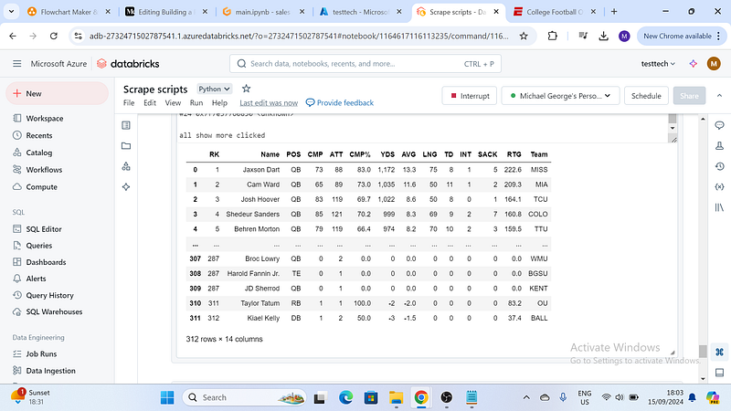

Ensure all data quality checks pass before saving DataFrames as Parquet to DBFS.

Now initially we used Great Expectations to run data quality checks but GE wasn’t working on Databricks most likely due to some dependency issues so I built a custom data quality check in Python. Here is a snippet of data quality checks for the player stats. Remember the full code is in the GitHub link at the bottom of the page.

df = dataframes
    check_results = []

    # Check 'Rk' (Rank) is not null and is an integer
    rk_null = df['Rank'].isnull().sum()
    rk_int = df['Rank'].dtype == 'int64'
    check_results.extend([
        {
            'check': "'Rank' not null",
            'result': 'Pass' if rk_null == 0 else 'Fail',
            'details': f"{rk_null} null values found"
        },
        {
            'check': "'Rank' is integer",
            'result': 'Pass' if rk_int else 'Fail',
            'details': f"Type is {df['Rank'].dtype}"
        }
    ])

    # Check 'Name' is not null and is a string
    name_null = df['Name'].isnull().sum()
    name_string = df['Name'].dtype == 'object'
    check_results.extend([
        {
            'check': "'Name' not null",
            'result': 'Pass' if name_null == 0 else 'Fail',
            'details': f"{name_null} null values found"
        },
        {
            'check': "'Name' is string",
            'result': 'Pass' if name_string else 'Fail',
            'details': f"Type is {df['Name'].dtype}"
        }
    ])

    # Check 'POS' is not null and is in a set of valid positions
    valid_positions = {
    "DL",
    "EDGE",
    "S",
    "QB",
    "RB",  # Running Back
    "FB",  # Fullback
    "WR",  # Wide Receiver
    "TE",  # Tight End
    "LT",  # Left Tackle
    "LG",  # Left Guard
    "C",   # Center
    "RG",  # Right Guard
    "RT",  # Right Tackle
    "DT",  # Defensive Tackle
    "DE",  # Defensive End
    "NT",  # Nose Tackle
    "LB",  # Linebacker
    "MLB", # Middle Linebacker
    "OLB", # Outside Linebacker
    "CB",  # Cornerback
    "FS",  # Free Safety
    "SS",  # Strong Safety
    "DB",  # Defensive Back (general term for CB and S)
    "OL",  # Offensive Line (general term for LT, LG, C, RG, RT)
    "PK",  # Placekicker
    "K",   # Kicker
    "P",   # Punter
    "LS",  # Long Snapper
    "KR",  # Kick Returner
    "PR",  # Punt Returner
    "G",   # Gunner (Special Teams)
    "H",   # Holder
    "KO"   # Kickoff Specialist
}  # Add more as needed
    pos_null = df['Position'].isnull().sum()
    pos_valid = df['Position'].isin(valid_positions).all()
    check_results.extend([
        {
            'check': "'Position' not null",
            'result': 'Pass' if pos_null == 0 else 'Fail',
            'details': f"{pos_null} null values found"
        },
        {
            'check': "'Position' is valid",
            'result': 'Pass' if pos_valid else 'Fail',
            'details': f"Invalid positions: {set(df['Position'].unique()) - valid_positions}"
        }
    ])

    # Check 'College' is not null and is a string
    College_null = df['College'].isnull().sum()
    College_string = df['College'].dtype == 'object'
    check_results.extend([
        {
            'check': "'College' not null",
            'result': 'Pass' if College_null == 0 else 'Fail',
            'details': f"{College_null} null values found"
        },
        {
            'check': "'College' is string",
            'result': 'Pass' if College_string else 'Fail',
            'details': f"Type is {df['College'].dtype}"
        }
    ])

    # Convert check results to a DataFrame
    results_df = pd.DataFrame(check_results)
    if (results_df['result'] == 'Pass').all():
        df.to_parquet(f"/dbfs/FileStore/player_stats_{url.rstrip('/').split('/')[-1]}.parquet")
        print("All rows in the column are 'pass'.")
    else:
        print(results_df)

The passing result as a dataframe;

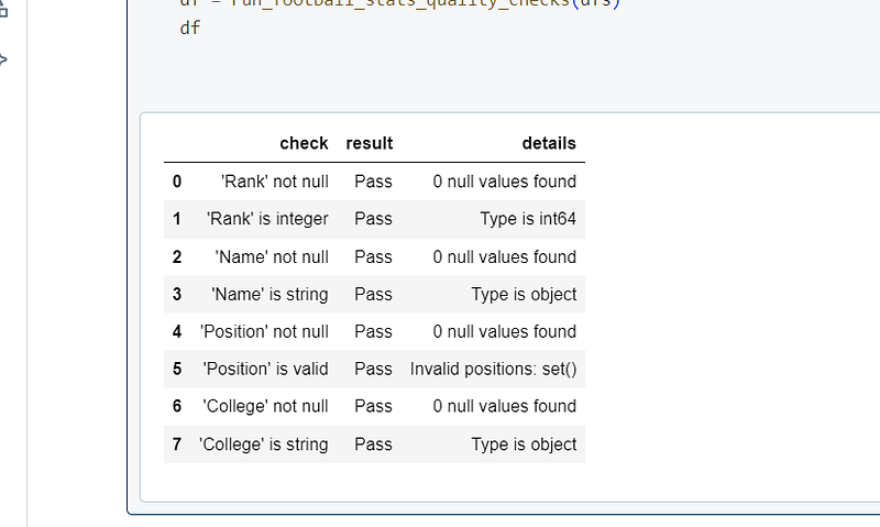
The code is a data quality validation script for a player stats DataFrame. It checks:

The 'Rank' column to ensure it has no null values and contains only integers.
The 'Name' column to verify that it is not null and contains only strings.
The 'Position' column to ensure it is not null and that all values match valid football positions.
The 'College' column to ensure it has no null values and consists of strings.

If all checks pass, the data is saved as a Parquet file to your DBFS; otherwise, it displays the results of the failed checks.

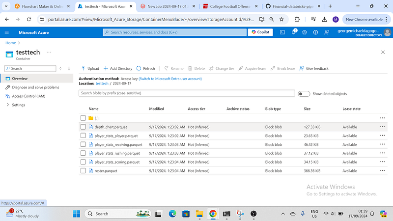
Save them in your Blob storage container in a new folder named after the current date.

To create a blob storage container go to your storage account and then to scroll down to containers and create a new container of your choice. I used testtech as my container name.

Now Our code that does the work;

from datetime import datetime
import os
import shutil

# Set up the blob storage account details
account_name = "testtech"
container_name = "testtech"
mount_point = "/mnt/testtech"
storage_key = "123-your---password---storage---key"

# The path to your Parquet files on DBFS
dbfs_parquet_path = 'dbfs:/FileStore'

# 1. Mount the blob storage container
def mount_blob_storage():
    if not any(mount.mountPoint == mount_point for mount in dbutils.fs.mounts()):
        dbutils.fs.mount(
            source = f"wasbs://{container_name}@{account_name}.blob.core.windows.net/",
            mount_point = mount_point,
            extra_configs = {f"fs.azure.account.key.{account_name}.blob.core.windows.net": storage_key}
        )
    print("Blob storage mounted.")

# 2. Create a new folder named with the current date
def create_new_folder():
    current_date = datetime.now().strftime("%Y-%m-%d")
    new_folder_path = os.path.join(mount_point, current_date)
    dbutils.fs.mkdirs(new_folder_path)
    print(f"New folder created: {new_folder_path}")
    return new_folder_path

# 3. Move Parquet files to the newly created folder
def move_parquet_files_to_blob(new_folder_path):
    files = dbutils.fs.ls(dbfs_parquet_path)
    
    for file in files:
        if file.path.endswith(".parquet"):
            dbutils.fs.mv(file.path, new_folder_path)
            print(f"Moved file {file.path} to {new_folder_path}")
    print("All Parquet files moved.")

# 4. Unmount the blob storage container
def unmount_blob_storage():
    dbutils.fs.unmount(mount_point)
    print("Blob storage unmounted.")

# 5. Remove the Parquet files from DBFS
def remove_parquet_files_from_dbfs():
    # List all files in the directory
    files = dbutils.fs.ls(dbfs_parquet_path)
    
    # Loop through the files and remove only the ones with '.parquet' extension
    for file in files:
        if file.name.endswith(".parquet"):
            dbutils.fs.rm(file.path)
            print(f"Removed Parquet file: {file.path}")

    print(f"All Parquet files removed from {dbfs_parquet_path}")

# Main function to run the whole process
def move_parquet_files():
    mount_blob_storage()  # Mount the blob storage
    new_folder_path = create_new_folder()  # Create a date-named folder
    move_parquet_files_to_blob(new_folder_path)  # Move files to the new folder
    unmount_blob_storage()  # Unmount the blob storage
    remove_parquet_files_from_dbfs()  # Delete parquet files from DBFS

# Run the process
move_parquet_files()

Here’s a summary of what the code does, step-by-step:

1. Mount the Blob Storage (mount_blob_storage function):

The code mounts an Azure Blob Storage container (specified by account_name and container_name) to a given mount_point (/mnt/testtech) in the Databricks File System (DBFS).
It checks if the container is already mounted by iterating through existing mounts.
If not already mounted, it uses the provided storage_key to mount the blob storage.

2. Create a New Folder with the Current Date (create_new_folder function):

The code generates a folder name based on the current date (in YYYY-MM-DD format) using the datetime.now() function.
It then creates this folder inside the mounted blob storage directory using the dbutils.fs.mkdirs method.
The folder path is returned for further operations.

3. Move Parquet Files to the New Folder (move_parquet_files_to_blob function):

The function lists all files located in the dbfs:/FileStore directory using dbutils.fs.ls.
It filters for files with the .parquet extension and moves them to the newly created folder in blob storage (returned by create_new_folder()).
Each file move is logged by printing the source and destination path.

4. Unmount Blob Storage (unmount_blob_storage function):

After the file move is complete, the blob storage container is unmounted using the dbutils.fs.unmount function.
The unmount operation is confirmed with a printed message.

5. Remove Parquet Files from DBFS (remove_parquet_files_from_dbfs function):

The function lists all files in the dbfs:/FileStore directory.
It identifies and removes files with the .parquet extension from the DBFS using the dbutils.fs.rm function.
A message confirming the deletion of each file is printed.

6. Main Function (move_parquet_files function):

This function runs the entire process in sequence:

Mounts the blob storage > Creates a folder with the current date in the blob storage >Moves Parquet files from DBFS to the new folder > Unmounts the blob storage > Removes the Parquet files from the DBFS.

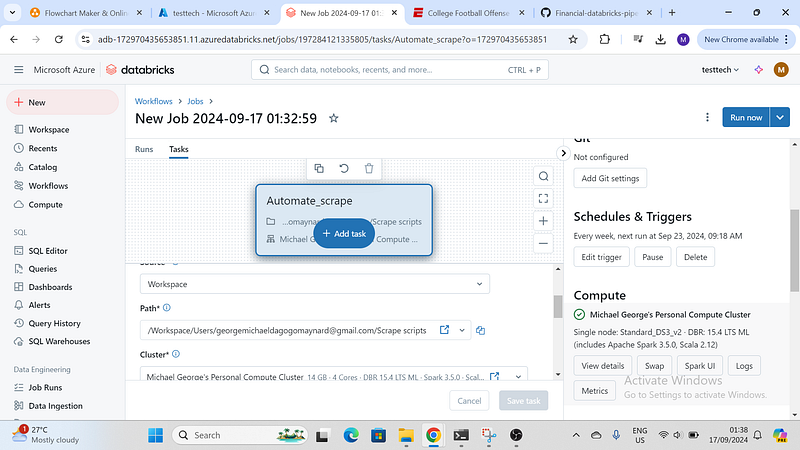
Schedule and automate script to run weekly.

Since we’ve done this before and it is quite straightforward;

Go to Workflows and create a new one.
Give it a name then choose the file for the Path
Choose the cluster that will be responsible for the Job runs then save task.
Create a trigger for it by choosing once a week.

That brings us to the end of our Batch Layer. Next the Speed layer.

STREAM LAYER

Develop a real-time streaming script that fetches live match data from the ESPN API and stores it efficiently in a Databricks SQL table.

We’ll be getting data from the ESPN API for scoreboard data which has no official documentation streamed with Spark Streaming.

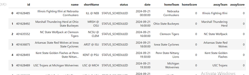
Just to see the output data let’s run a quick code on our local machine first.

import requests
import json
from datetime import datetime
import pandas as pd

url = "https://site.api.espn.com/apis/site/v2/sports/football/college-football/scoreboard"
response = requests.get(url, timeout=10)
response.raise_for_status()  # Raise an exception for bad status codes
data = response.json()

matches = []
for event in data.get('events', []):
    match = {
        'id': event['id'],
        'name': event['name'],
        'shortName': event['shortName'],
        'status': event['status']['type']['name'],
        'date': datetime.strptime(event['date'], "%Y-%m-%dT%H:%MZ"),
        'homeTeam': event['competitions'][0]['competitors'][0]['team']['displayName'],
        'homeScore': int(event['competitions'][0]['competitors'][0]['score']),
        'awayTeam': event['competitions'][0]['competitors'][1]['team']['displayName'],
        'awayScore': int(event['competitions'][0]['competitors'][1]['score'])
    }
    matches.append(match)
df = pd.DataFrame(matches)
df

Output;

To Databricks with our full stream code;

# Databricks notebook source
from pyspark.sql import SparkSession
from pyspark.sql.functions import *
from pyspark.sql.types import *
import requests
import json
from datetime import datetime

# Initialize Spark Session with Delta support
spark = SparkSession.builder \
    .appName("ESPNCollegeFootballStreaming") \
    .config("spark.sql.extensions", "io.delta.sql.DeltaSparkSessionExtension") \
    .config("spark.sql.catalog.spark_catalog", "org.apache.spark.sql.delta.catalog.DeltaCatalog") \
    .getOrCreate()

# Define the schema for the DataFrame
schema = StructType([
    StructField("id", StringType(), True),
    StructField("name", StringType(), True),
    StructField("shortName", StringType(), True),
    StructField("status", StringType(), True),  # Status is string, not boolean
    StructField("date", TimestampType(), True),
    StructField("homeTeam", StringType(), True),
    StructField("homeScore", IntegerType(), True),
    StructField("awayTeam", StringType(), True),
    StructField("awayScore", IntegerType(), True)
])

# Function to fetch data from ESPN API
def fetch_espn_data():
    try:
        url = "https://site.api.espn.com/apis/site/v2/sports/football/college-football/scoreboard"
        response = requests.get(url, timeout=10)
        response.raise_for_status()  # Raise an exception for bad status codes
        data = response.json()
        
        matches = []
        for event in data.get('events', []):
            try:
                match = {
                    'id': event['id'],
                    'name': event['name'],
                    'shortName': event['shortName'],
                    'status': event['status']['type']['name'],  # Treat status as string
                    'date': datetime.strptime(event['date'], "%Y-%m-%dT%H:%MZ"),
                    'homeTeam': event['competitions'][0]['competitors'][0]['team']['displayName'],
                    'homeScore': int(event['competitions'][0]['competitors'][0]['score']),
                    'awayTeam': event['competitions'][0]['competitors'][1]['team']['displayName'],
                    'awayScore': int(event['competitions'][0]['competitors'][1]['score'])
                }
                matches.append(match)
            except (KeyError, IndexError, ValueError) as e:
                print(f"Error processing event: {e}")
                continue
        
        return matches
    except requests.RequestException as e:
        print(f"Error fetching data from ESPN API: {e}")
        return []

# Function to process each batch of streaming data
def process_batch(df, epoch_id):
    try:
        # Fetch ESPN data
        espn_data = fetch_espn_data()
        
        if not espn_data:
            print(f"No data to process for batch {epoch_id}")
            return
        
        # Convert the data to a Spark DataFrame
        spark_df = spark.createDataFrame(espn_data, schema)
        
        # Write the DataFrame to a Delta table
        delta_table_name = "college_football_matches"
        spark_df.write.format("delta").mode("overwrite").saveAsTable(delta_table_name)
        
        print(f"Batch {epoch_id} processed. Data written to SQL table {delta_table_name}")
    except Exception as e:
        print(f"Error processing batch {epoch_id}: {e}")

# Create a streaming DataFrame
streaming_df = spark.readStream \
    .format("rate") \
    .option("rowsPerSecond", 1) \
    .load()

# Start the streaming query
query = streaming_df.writeStream \
    .foreachBatch(process_batch) \
    .outputMode("update") \
    .trigger(processingTime='1 minutes') \
    .start()

# Wait for the streaming to finish
query.awaitTermination()

This code sets up a real-time data pipeline that fetches live match data from the ESPN College Football API and stores it in a Delta table on Databricks. Here’s what each part does:

Initialize Spark Session with Delta Support: The script configures a Spark session with Delta Lake support to enable efficient data storage and management using Delta tables.
Define Schema: It defines a schema for the data, including fields like id, name, status, date, homeTeam, homeScore, awayTeam, and awayScore.
Fetch Data from ESPN API: The fetch_espn_data function makes a request to the ESPN API and processes the response to extract match details like team names, scores, status, and match date. It handles potential errors during data extraction and skips invalid data.
Process Streaming Data: The process_batch function is triggered with each streaming batch. It fetches the latest ESPN match data, converts it into a Spark DataFrame, and writes the data to a Delta table (college_football_matches) in overwrite mode, ensuring that the table always has the latest data.
Create a Streaming DataFrame: A simulated streaming DataFrame (streaming_df) is created with rows generated at a rate of 1 row per second. This simulates the ingestion of data at regular intervals.
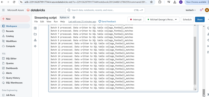
Start the Streaming Query: The writeStream method is used to process each batch using the process_batch function. The query triggers every minute to fetch and process new data. It continuously runs the process to fetch live data, write to Delta, and refresh the SQL table.

Output;

Develop a Databricks dashboard to visualize live match data in real-time.

Now understand this, I used the dashboarding tool on Databricks with only the table visual function. While your streaming code is still running, this visualization part is optional as we are doing this just to see the data change in real time.

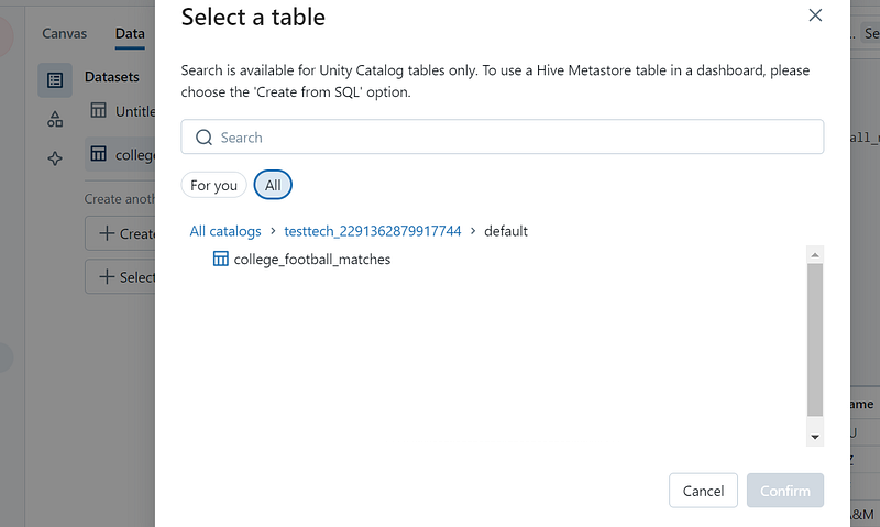
Click on Dashboard(on the sidebar) and Create a new dashboard where you’ll need to choose between ‘Create from SQL’ or ‘Select a Table’, click on the latter and locate your delta table with the name college_football_matches .

We can use query our table to limit the data we’re going to work with and in this case, we just need matches with the status column as STATUS_IN_PROGRESS. You will need to start a Serverless SQL before you can run the query.

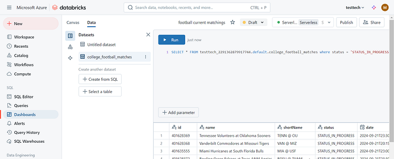
SELECT * FROM testtech.default.college_football_matches where status = 'STATUS_IN_PROGRESS'

Next is to simply click on the table visual icon in the canvas tab then select the columns you want there.

SERVING LAYER

This part of the project is your opportunity to be creative and take initiative, without relying on step-by-step guidance.

Provision a PostgreSQL database on Azure Portal.

It’s very straightforward, but use development not production, to reduce potential cost.

Design and implement a normalized database schema.

If I wanted to create a normalized data model for our data, the player stats CSV would have separate tables in the database with no connections for now, but the depth chart and roster CSV would be normalized like this.

Depth Chart has these columns; Position, field_pos, team_name, String Order, Player Number, First Name Last Name, and School year.

Roster CSV has these columns; Player Number, Position, height, Weight, Class, High School, Hometown, First Name, Last Name, and team_name.

TEAM Table:

Contains unique team information
Primary Key: team_id
Fields: team_name

PLAYER Table:

Contains all player information
Primary Key: player_id
Foreign Key: team_id (references TEAM table)
Fields: First Name, Last Name, Number, Position, Height, Weight, Class, High School, Hometown

DEPTH_CHART Table:

Represents the depth chart information
Primary Key: depth_chart_id
Foreign Keys: player_id (references PLAYER table), team_id (references TEAM table)
Fields: position, field_pos, order

SCHOOL_YEAR Table:

Contains unique school years
Primary Key: school_year_id
Fields: FR, SO, JR, SR

PLAYER_SCHOOL_YEAR Table:

Represents the many-to-many relationship between players and school years
Primary Key: player_school_year_id
Foreign Keys: player_id (references PLAYER table), school_year_id (references SCHOOL_YEAR table)

Note: the above model can be revised, changed, or even improved upon. You’re advised to create the primary keys and separate these into separate dataframes or files before pushing them to your database.

This normalized structure offers several benefits:

Eliminates data redundancy by separating team, player, and depth chart information.
Allows for multiple depth chart entries per player (e.g., if a player has multiple positions).
Supports tracking players across multiple school years without duplicating player information.
Maintains data integrity through proper use of primary and foreign keys.

To use this model:

Each unique team would have one entry in the TEAM table.
Each player would have one entry in the PLAYER table, regardless of how many positions they play or years they’ve been on the team.
The DEPTH_CHART table would have an entry for each player’s position in the depth chart.
The SCHOOL_YEAR table would list all relevant school years.
The PLAYER_SCHOOL_YEAR table would link players to each school year they’re associated with.

Migrate the relevant data into the PostgreSQL database.

This is your time to be creative, whichever data model you come up with, create tables accordingly and push to the database.

Conclusion

You don’t learn much by CTRL C CTRL V, you learn by doing the work and thinking critically on how to solve issues.

Link to GitHub Repository: https://github.com/George-Michael-Dagogo/Databricks_Lambda_Architecture

References

Streaming on Azure Databricks - Azure Databricks

Learn about streaming, incremental, and real-time workloads powered by Structured Streaming on Azure Databricks.

learn.microsoft.com

Structured Streaming - PySpark master documentation

pyspark.sql.SparkSession.builder.getOrCreate

api-docs.databricks.com

Selenium chrome driver on databricks driver On the databricks community, I see repeated problems…

Selenium chrome driver on databricks driver On the databricks community, I see repeated problems regarding the selenium…

community.databricks.com