Building a Q-table Reinforement Learning Agent with Captain Picard

Is it possible to combine reinforcement learning via q-tables with a crazy quest for Captain Jean-Luc Picard to find all the earl grey tea? Engage!

If someone had told me that I’d be spending a rainy afternoon building a demo of reinforcement learning via ‘q-tables’ by sending Captain Picard on a demenated chase through an old folks home for earl grey tea, I’d have called them a lunatic.

Yet, here we are.

(This is what happens when I’m on annual leave for a while and I start to get bored…)

If you cast your mind back to August ’23, I spent some time writing a guide about the basics of reinforcement learning:

In it, we took a look at the ‘many armed bandit’ problem, and compared different ways to maximise our rewards progressing through random selection, to greedy selection and finally to using greedy epsilon. It was — for me at least — a lot of fun! But it was really only scratching the very surface of the reinforcement learning itch. Once you start reading about the wider world of ‘RL’ you find that it’s a deep and complex world of different algorithms, methodologies and frameworks each with their own strengths and weaknesses when it comes to teaching a computer how to maximise its rewards.

In this follow-up piece, we’re going to go a level deeper into the world of reinforcement learning, and explore one of the more complex — but hopefully interesting — methods for using reinforcement learning to solve problems, culminating in the build of our very own reinforement learning experiement! If you’re willing to stick with me through the rest of the article, you’ll even be treated to a small tech demo of reinforcement learning you can experience in your own browser.

Q who?

“Predicting the future isn’t magic, it’s artificial intelligence.” — Dave Waters

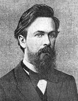
We’re going to be learning about a particular mechansim for reinforcement learning called ‘Q-learning’, and to understand what that is we need to go all the way back to 1989 and an enterprising Professor by the name of Christoper Watkins.

Watkins has been a critital contributor to the AI/ML enteprise having authored or co-authored a wealth of papers on machine learning (including a 2022 study that draws similarities between the way large language models and humans intepret text) but it’s a paper he wrote in 1989 introducing the concept of ‘Q-learning’ that we’re going to focus on today.

In the words of the paper, “Q-learning (Watkins, 1989) is a simple way for agents to learn how to act optimally in controlled Markovian domains”. (More on Markovian domains later)

At its heart, Q-learning — like other reinforcement learning methods and algorithms — is a way of helping an agent to understand its environment to maximise a reward in a given scenario. If we think back to our first piece on reinforcement learning, we imagined the ‘RL loop’ as follows:

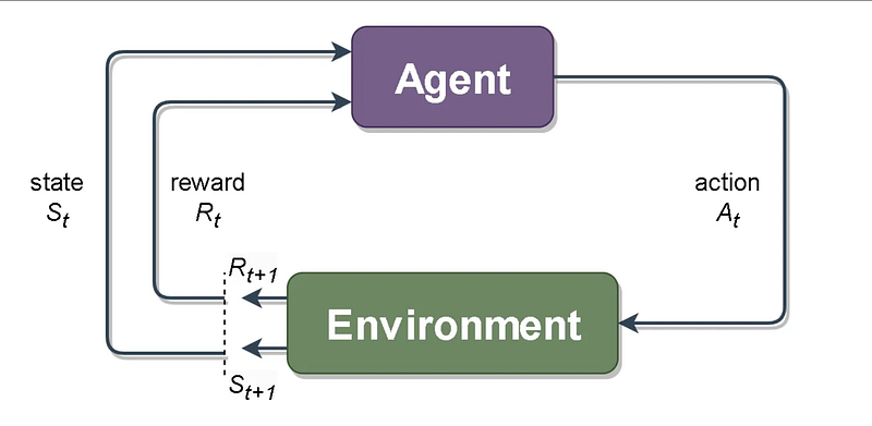
And the same diagram holds true for Q-learning. In the abstract we have an agent which takes actions in an environment to obtain a reward, and in a real world use case we might employ it for online marketing to optimise showing customers the most relevent ads for their buying habits (the reward being when the customer clicks on an ad).

In Q learning, an agent tries an action at a particular state, and evaluates its consequences in terms of the immediate reward or penalty it receives and its estimate of the value of the state to which it is taken. By trying all actions in all states repeatedly, it learns which are best overall, judged by long-term discounted reward

In order to store information about the value of taking actions within the environment, Q-learning employs a ‘Q-table’.

Think of the q table as just that, a look up table of columns and rows representing the state and actions possible in the environment.

Each ‘cell’ in your q table is initially set as 0 (which you can think of as ‘unexplored’) but as the agent explores it will update the q-table with the rewards obtained for each combination of state and action. Over time the idea is the agent will converge on the best actions to take in the environment to maximise the reward by leveraging the information being continually updated in the q table.

To put this in perspective for our previous articles 3 armed bandit problem, the initial q-table might look like this:

+-------+-------+-------+-------+
| State | Arm 1 | Arm 2 | Arm 3 |
+-------+-------+-------+-------+
|   1   |   0   |   0   |   0   |
+-------+-------+-------+-------+

There’s really only one state (pulling the lever) when it comes to a slot machine, and there are 3 machines in the 3 armed bandit problem, so we end up with the above. After a few pulls of the slots, we might end up with some reward values:

+-------+-------+-------+-------+
| State | Arm 1 | Arm 2 | Arm 3 |
+-------+-------+-------+-------+
|   1   |   0.5 |   1   |   4   |
+-------+-------+-------+-------+

When the agent is in a state, it looks at the row in the Q-table for that state and in most cases chooses the action with the highest Q-value in that row (the best action it knows so far). Factors like the ‘exploration rate’ (how often the agent will choose to explore a new action versus exploit a known good action) and ‘exploration decay’ (the rate at which the agent will eventually converge on and stick to what it considers the maximal reward path) will influence how much the agent relies only on the value it finds in the Q-table.

The formula for interacting with the Q-table (called the ‘Bellman’ equation) looks as follows:

New Q-value=Old Q-value+Learning Rate×(Reward+Discount×Best Future Q-value−Old Q-value)

The idea of the Bellman equation is that the value of a state-action pair is updated based not only on the immediate reward but also on the best expected future rewards, adjusted by the learning rate. But what about the past rewards? The history of what came before?

The role of the Markov property

It’s important to note that the use of a q-table and the q-learning method for reinforcement learning is best suited to environments that follow the ‘Markov’ property.

What’s that?

Well in essence an environment is considered ‘Markov’ (from the Russian mathematician, Andrey Markov) when the future state of an agent within the environment depends only on the current state and the action taken in that state, not on the sequence of events or states that preceded it. Basically, the past doesn’t matter, only the here and now and the immediate future when it comes to converging on the best rewards.

An example of a Markov environment is a connect four board. Each time you make a move in connect four, it’s really only relevent the state of the board at the time, it doesn’t matter what someone did 5 moves ago (well, it did matter at the time, but in order to play a move you just need to know the current state of the board and all the pieces in play.)

For a good example of a non Markov environment you could consider something like a game of Poker. There’s not only the current cards and betting pool, but there’s the history of the opponents bets in the context of bluffing etc. that could alter your strategy in order to play the current and future hands.

Reinforcement learning has mechanisms for dealing with Markov and non-Markov environments, but Q-learning is designed for the former.

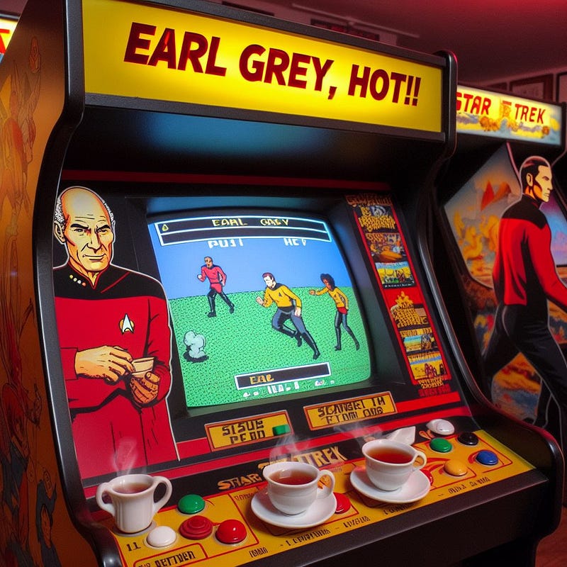
Earl Grey, HOT!

So now the moment you’ve been waiting for, how on earth does all this fit in with Captain Jean-Luc Picard of Star Trek: The Next Generation fame? Well, we’re going to use the aforementioned Starfleet captain and his (in)famous love of Earl Grey tea to demonstrate our own implementation of Q-learning!

For that, we’ve decided to design a simple arcade game based in the Star Trek universe called ‘Earl Grey, HOT!’.

In order to build our RL based game, we’re going to need a couple of things. You won’t need to build any of this yourself as I’m going to give you the GitHub repository at the end, this is more just to bring you along for the journey as I put this together. Anyway, for the experiment, I went with:

• Phaser (Web based Game development toolkit). I picked this so I could quickly prototype something that could be hosted in the browser for each of demonstration. You can learn more about Phaser here https://phaser.io/
• JavaScript (as we’re building something browser/client based, we’re going to use plain old vanilla JavaScript).
• AWS AppRunner (This is just for hosting our final solution to show you the demo, you won’t need any knowledge of AppRunner. There is an amazingly simple and effective integration connection that can be established between GitHub and AWS AppRunner that makes deployments simple, hence it’s my pick. More on that here https://docs.aws.amazon.com/apprunner/latest/dg/service-source-code.html

My ‘storyline’ in so far as I have one, is that poor old Picard has been infected with some kind of space pathogen. This virus has overridden the logic and decisions centers of his brain and caused him to go into an animal-like frenzy of lust for — you guessed it — earl grey tea. As a result, he’s been spotted ransacking local retirement homes on the search for more and more of that earl grey goodness. This will form the core of our:

• Agent (Captain Picard)
• Environment (Old folks home, in our case an 8 * 8 grid)
• Goal (cup of earl grey)
• Some Obstacles (nursing staff at the retirement home that block Picards progress!)

For our application, we’re keeping things super simple. There’s an index.html for displaying our game, a game.js containing the RL logic, a node.js script (server.js) to host our game, and some .png assets. You find all of the finished assets in the following repository ready for your viewing pleasure:

Our Web UI also has some Reinforcement Learning parameters you can tweak to see if you can affect the performance of our agent! They are:

• Learning Rate — The rate at which the agent learns from its experiences. A higher learning rate means the agent will learn faster, but it may also be more prone to overfitting.
• Discount Factor — The discount factor determines how much the agent values future rewards. A higher discount factor means the agent will value future rewards more, and vice versa.
• Exploration Rate — The exploration rate determines how often the agent will explore new actions. A higher exploration rate means the agent will explore more often, and vice versa.
• Exploration Decay — The exploration decay determines how quickly the exploration rate will decrease over time. A higher exploration decay means the exploration rate will decrease faster, and vice versa.

Rather than go through all the JavaScript code bit by bit, we’re going to focus on the bits that deal most specifically with our implementation of reinforcement learning. For information on setting up the basics of a Phaser game (sprites, environment and so on) refer to the Phaser website.

Because we’re using Q-learning, we’ll need to create a q-table, but our q-table needs to be more complex than the one we touched on earlier. If you think about our RL environment, you have an 8 by 8 grid, so that’s 64 different states. Additionally, Picard can move either up, down, left or right from each of these grid tiles, so that brings us to 8 by 8 by 4. For this, we’ll need a 3 dimensional array!

To do this in our game.js we’re creating the q-table as follows:

function create() {
    // Create my qtable which is gridSize x gridSize x 4 (the 4 is the number of actions)
    qTable = Array(gridSize).fill().map(() => Array(gridSize).fill().map(() => Array(4).fill(0)));

Basically we’re creating an array with a length of the grid, then we’re creating an array inside that array where each element is an array the length of the grid, then we’re creating an array inside THAT array so that each element contains an array for the 4 action states.

And what’s going to happen in our game? Well, the guts of the decision making process is taken care of in our function update(time) method.

It’s here that our agent decides on an action, takes it, has the reward updated, updates the q-table and progress on until the goal is met. There’s a lot of code within update(time) just deals with updating positions and rendering sprites or text, but two core parts to examine are function chooseAction(position), and function takeAction(position, action).

Here is our choose action method:

function chooseAction(position) {
    var action;

    // Avoid the action that would reverse the last move
    var avoidActions = lastActions(); // Function to get last few actions to avoid

    if (Math.random() < explorationRate) {
        do {
            action = Math.floor(Math.random() * 4); // Explore
        } while (avoidActions.includes(action));
    } else {
        // Exploit the best-known action, avoiding the reverse of the last actions if possible
        var currentQValues = [...qTable[position.y][position.x]]; // Clone the current Q-values
        avoidActions.forEach(a => currentQValues[a] = Math.min(...currentQValues)); // Discourage reverse actions
        var maxQValue = Math.max(...currentQValues);
        action = currentQValues.indexOf(maxQValue);
    }

    updateLastActions(action); // Update the last actions taken
    return action;
}

We use a little randomness in our choice of whether to explore (seek out new areas) or exploit (go with known good rewards) but you can see it’s controlled to a degree based on the value of our explorationRate.

If we decide to explore, we’ll pick a random up/down/left/right action (but you’ll notice I did have to add a check not to choose from a series of the very most recent actions. This helped to stop the agent from essentially getting stuck in an infinite loop of going back and forth betwen say, 2 tiles).

If we decide to exploit, then we’ll rely on our Q-table to tell us what that best known action is (which gets better and more ‘known’ as time goes on and more moves are made). We’ll then take our action, move, and do things like check whether we’ve encountered a nurse, a normal space in our grid, or the goal itself — delicious earl grey tea!

In our takeAction() method, we’ve essentially built a ‘reward’ function, in that we’ll move Picard around (if possible) and provide a positive reward if we’ve found our goal, or a slightly negative reward (cumulative) if we’ve hit an obstacle:

function takeAction(position, action) {
    var reward = -0.01;
    var newPosition = { x: position.x, y: position.y };

    // Check if the new position is valid (not an obstacle and within grid bounds)
    function isValidMove(newX, newY) {
        if (newX < 0 || newY < 0 || newX >= gridSize || newY >= gridSize) {
            return false; // Out of grid bounds
        }
        return !obstacles.some(obstacle => obstacle.x / tileSize === newX && obstacle.y / tileSize === newY);
    }

    // Determine new position based on the action
    switch (action) {
        case 0: // Up
            if (isValidMove(position.x, position.y - 1)) newPosition.y -= 1;
            break;
        case 1: // Right
            if (isValidMove(position.x + 1, position.y)) newPosition.x += 1;
            break;
        case 2: // Down
            if (isValidMove(position.x, position.y + 1)) newPosition.y += 1;
            break;
        case 3: // Left
            if (isValidMove(position.x - 1, position.y)) newPosition.x -= 1;
            break;
    }

    if (newPosition.x !== position.x || newPosition.y !== position.y) {
        // Update agent position if it's a valid move
        agentPosition = newPosition;

        if (agentPosition.x === goalPosition.x && agentPosition.y === goalPosition.y) {
            reward = 1; // Reward for reaching the goal
        }
    } else {
        // Invalid move (either out of bounds or into an obstacle)
        reward -= 0.1;
    }

    return reward;
}

Once we’ve decided and moved Picard, we need to update the q-table as follows:

function updateQTable(position, action, reward) {
    var nextState = agentPosition;
    var maxQValueNextState = Math.max(...qTable[nextState.y][nextState.x]);
    qTable[position.y][position.x][action] += learningRate * (reward + discountFactor * maxQValueNextState - qTable[position.y][position.x][action]);
}

This is the JavaScript implementation of the following update rule for the Q-table:

Q(state,action)←Q(state,action)+α×(reward+γ×maxa​Q(nextState,a)−Q(state,action))

Or put simply: New Score = Old Score + Learning Factor × (Recent Points + Future Potential — Old Score).

Besides choosing an action, taking it and updating the q-table, there are a couple of other actions we take in our update method and these relate to the weighting for whether the agent should explore vs exploit.

Firstly, we slowly (depending on our decay rate) reduce the amount of exploration the agent does each step so we can converge on the maximum best reward path:

explorationRate = Math.max(explorationRate - explorationDecay, 0.01);

But in addition to this, I had to add a small adjustment in the update method that temporarily increases or boosts the potential decision to explore if for some reason the agent appears ‘stuck’.

        if (samePositionCount > 3) {
            explorationRate = Math.min(explorationRate + 0.1, 1.0);
            samePositionCount = 0;  // Reset the counter
        }

Before this, the agent would often get stuck in a loop somewhere, but with the addition it gives him a bit of a ‘nudge’ if he gets stuck and seems to be in the same position(s) for a little while. The change is temporary and only until the agent gets moving again.

The game measures the reward each time Picard gets to his precious earl grey, and considers the experiment complete/won when he converges on the maximum reward possible for 5 consecutive attempts. At this point we figure the agent is as ‘fitted’ to the task as is reasonably possible.

The finished product? The incredibly awesome (I know, I know — it’s pretty hokey, but still fun I hope!) ‘Earl Grey, HOT1’ game, that you can try out at:

https://earlgreyhot.org/

Have fun, adjust the parameters, and see how few attempts you can tweak the agent to complete his earl grey hunt with! As a stretch goal, I invite someone to update the source code to include the ability to adjust the various rewards (positive and negative, or even create some new ones?) and allow users to see what impact that has on the performance of the agent?

Hopefully you found this an entertaining — and altogether Trekky — way to engage with the concept of reinforcement learning via q-learning and as always, if you enjoyed this article feel free to leave a clap and/or a comment — until next time!