Building A Logistic Regression in Python, Step by Step

Logistic Regression is a Machine Learning classification algorithm that is used to predict the probability of a categorical dependent variable. In logistic regression, the dependent variable is a binary variable that contains data coded as 1 (yes, success, etc.) or 0 (no, failure, etc.). In other words, the logistic regression model predicts P(Y=1) as a function of X.

Logistic Regression Assumptions

• Binary logistic regression requires the dependent variable to be binary.
• For a binary regression, the factor level 1 of the dependent variable should represent the desired outcome.
• Only the meaningful variables should be included.
• The independent variables should be independent of each other. That is, the model should have little or no multicollinearity.
• The independent variables are linearly related to the log odds.
• Logistic regression requires quite large sample sizes.

Keeping the above assumptions in mind, let’s look at our dataset.

Data

The dataset comes from the UCI Machine Learning repository, and it is related to direct marketing campaigns (phone calls) of a Portuguese banking institution. The classification goal is to predict whether the client will subscribe (1/0) to a term deposit (variable y). The dataset can be downloaded from here.

import pandas as pd
import numpy as np
from sklearn import preprocessing
import matplotlib.pyplot as plt 
plt.rc("font", size=14)
from sklearn.linear_model import LogisticRegression
from sklearn.model_selection import train_test_split
import seaborn as sns
sns.set(style="white")
sns.set(style="whitegrid", color_codes=True)

The dataset provides the bank customers’ information. It includes 41,188 records and 21 fields.

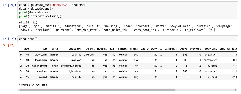
Input variables

1. age (numeric)
2. job : type of job (categorical: “admin”, “blue-collar”, “entrepreneur”, “housemaid”, “management”, “retired”, “self-employed”, “services”, “student”, “technician”, “unemployed”, “unknown”)
3. marital : marital status (categorical: “divorced”, “married”, “single”, “unknown”)
4. education (categorical: “basic.4y”, “basic.6y”, “basic.9y”, “high.school”, “illiterate”, “professional.course”, “university.degree”, “unknown”)
5. default: has credit in default? (categorical: “no”, “yes”, “unknown”)
6. housing: has housing loan? (categorical: “no”, “yes”, “unknown”)
7. loan: has personal loan? (categorical: “no”, “yes”, “unknown”)
8. contact: contact communication type (categorical: “cellular”, “telephone”)
9. month: last contact month of year (categorical: “jan”, “feb”, “mar”, …, “nov”, “dec”)
10. day_of_week: last contact day of the week (categorical: “mon”, “tue”, “wed”, “thu”, “fri”)
11. duration: last contact duration, in seconds (numeric). Important note: this attribute highly affects the output target (e.g., if duration=0 then y=’no’). The duration is not known before a call is performed, also, after the end of the call, y is obviously known. Thus, this input should only be included for benchmark purposes and should be discarded if the intention is to have a realistic predictive model
12. campaign: number of contacts performed during this campaign and for this client (numeric, includes last contact)
13. pdays: number of days that passed by after the client was last contacted from a previous campaign (numeric; 999 means client was not previously contacted)
14. previous: number of contacts performed before this campaign and for this client (numeric)
15. poutcome: outcome of the previous marketing campaign (categorical: “failure”, “nonexistent”, “success”)
16. emp.var.rate: employment variation rate — (numeric)
17. cons.price.idx: consumer price index — (numeric)
18. cons.conf.idx: consumer confidence index — (numeric)
19. euribor3m: euribor 3 month rate — (numeric)
20. nr.employed: number of employees — (numeric)

Predict variable (desired target):

y — has the client subscribed a term deposit? (binary: “1”, means “Yes”, “0” means “No”)

The education column of the dataset has many categories and we need to reduce the categories for a better modelling. The education column has the following categories:

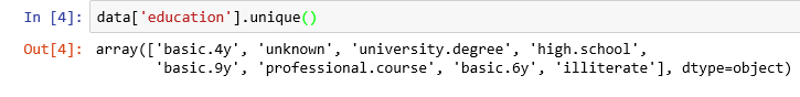
Let us group “basic.4y”, “basic.9y” and “basic.6y” together and call them “basic”.

data['education']=np.where(data['education'] =='basic.9y', 'Basic', data['education'])
data['education']=np.where(data['education'] =='basic.6y', 'Basic', data['education'])
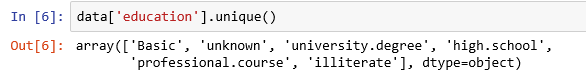
data['education']=np.where(data['education'] =='basic.4y', 'Basic', data['education'])

After grouping, this is the columns:

Data exploration

count_no_sub = len(data[data['y']==0])
count_sub = len(data[data['y']==1])
pct_of_no_sub = count_no_sub/(count_no_sub+count_sub)
print("percentage of no subscription is", pct_of_no_sub*100)
pct_of_sub = count_sub/(count_no_sub+count_sub)
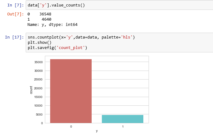
print("percentage of subscription", pct_of_sub*100)

percentage of no subscription is 88.73458288821988

percentage of subscription 11.265417111780131

Our classes are imbalanced, and the ratio of no-subscription to subscription instances is 89:11. Before we go ahead to balance the classes, let’s do some more exploration.

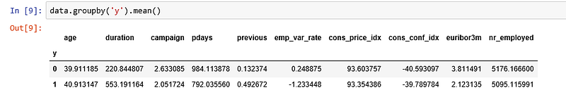
Observations:

• The average age of customers who bought the term deposit is higher than that of the customers who didn’t.
• The pdays (days since the customer was last contacted) is understandably lower for the customers who bought it. The lower the pdays, the better the memory of the last call and hence the better chances of a sale.
• Surprisingly, campaigns (number of contacts or calls made during the current campaign) are lower for customers who bought the term deposit.

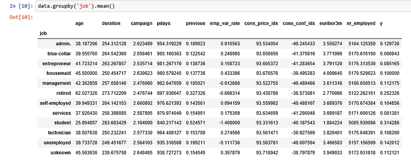
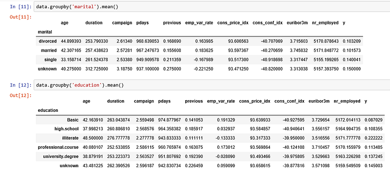
We can calculate categorical means for other categorical variables such as education and marital status to get a more detailed sense of our data.

Visualizations

%matplotlib inline
pd.crosstab(data.job,data.y).plot(kind='bar')
plt.title('Purchase Frequency for Job Title')
plt.xlabel('Job')
plt.ylabel('Frequency of Purchase')
plt.savefig('purchase_fre_job')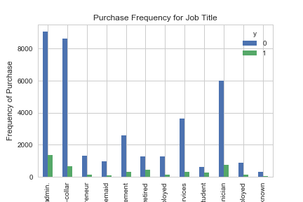

The frequency of purchase of the deposit depends a great deal on the job title. Thus, the job title can be a good predictor of the outcome variable.

table=pd.crosstab(data.marital,data.y)
table.div(table.sum(1).astype(float), axis=0).plot(kind='bar', stacked=True)
plt.title('Stacked Bar Chart of Marital Status vs Purchase')
plt.xlabel('Marital Status')
plt.ylabel('Proportion of Customers')
plt.savefig('mariral_vs_pur_stack')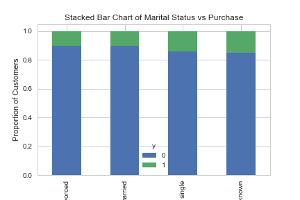

The marital status does not seem a strong predictor for the outcome variable.

table=pd.crosstab(data.education,data.y)
table.div(table.sum(1).astype(float), axis=0).plot(kind='bar', stacked=True)
plt.title('Stacked Bar Chart of Education vs Purchase')
plt.xlabel('Education')
plt.ylabel('Proportion of Customers')
plt.savefig('edu_vs_pur_stack')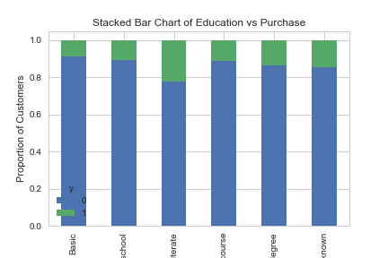

Education seems a good predictor of the outcome variable.

pd.crosstab(data.day_of_week,data.y).plot(kind='bar')
plt.title('Purchase Frequency for Day of Week')
plt.xlabel('Day of Week')
plt.ylabel('Frequency of Purchase')
plt.savefig('pur_dayofweek_bar')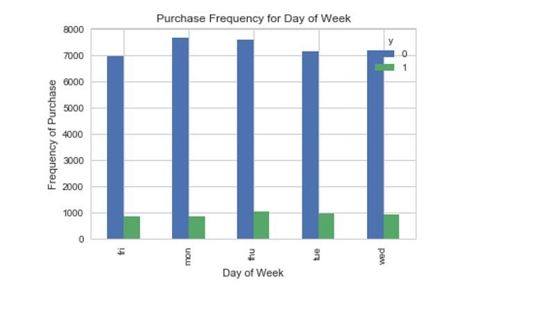

Day of week may not be a good predictor of the outcome.

pd.crosstab(data.month,data.y).plot(kind='bar')
plt.title('Purchase Frequency for Month')
plt.xlabel('Month')
plt.ylabel('Frequency of Purchase')
plt.savefig('pur_fre_month_bar')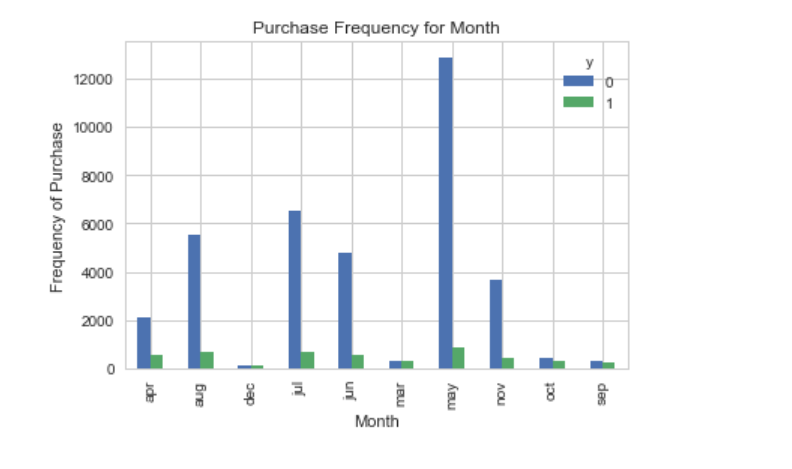

Month might be a good predictor of the outcome variable.

data.age.hist()
plt.title('Histogram of Age')
plt.xlabel('Age')
plt.ylabel('Frequency')
plt.savefig('hist_age')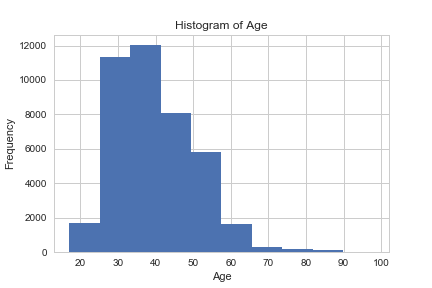

Most of the customers of the bank in this dataset are in the age range of 30–40.

pd.crosstab(data.poutcome,data.y).plot(kind='bar')
plt.title('Purchase Frequency for Poutcome')
plt.xlabel('Poutcome')
plt.ylabel('Frequency of Purchase')
plt.savefig('pur_fre_pout_bar')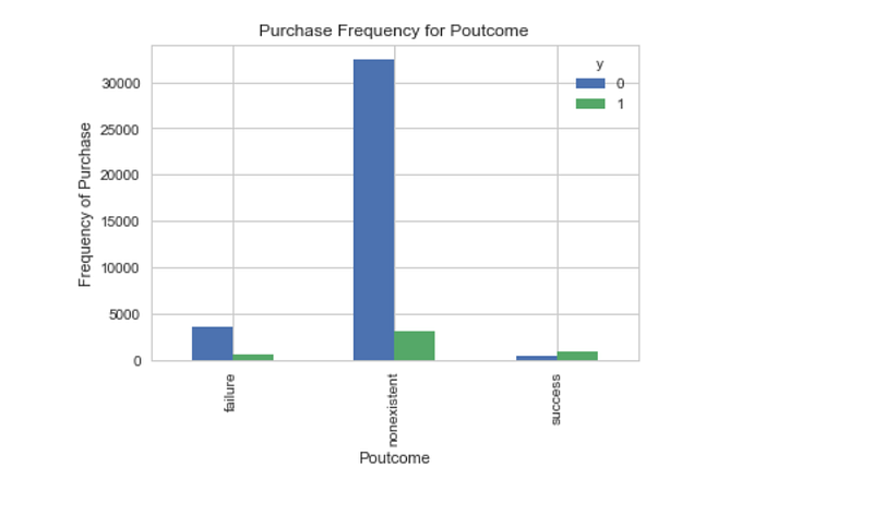

Poutcome seems to be a good predictor of the outcome variable.

Create dummy variables

That is variables with only two values, zero and one.

cat_vars=['job','marital','education','default','housing','loan','contact','month','day_of_week','poutcome']
for var in cat_vars:
    cat_list='var'+'_'+var
    cat_list = pd.get_dummies(data[var], prefix=var)
    data1=data.join(cat_list)
    data=data1

cat_vars=['job','marital','education','default','housing','loan','contact','month','day_of_week','poutcome']
data_vars=data.columns.values.tolist()
to_keep=[i for i in data_vars if i not in cat_vars]

Our final data columns will be:

data_final=data[to_keep]
data_final.columns.values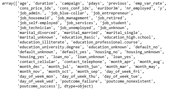

Over-sampling using SMOTE

With our training data created, I’ll up-sample the no-subscription using the SMOTE algorithm(Synthetic Minority Oversampling Technique). At a high level, SMOTE:

1. Works by creating synthetic samples from the minor class (no-subscription) instead of creating copies.
2. Randomly choosing one of the k-nearest-neighbors and using it to create a similar, but randomly tweaked, new observations.

We are going to implement SMOTE in Python.

X = data_final.loc[:, data_final.columns != 'y']
y = data_final.loc[:, data_final.columns == 'y']

from imblearn.over_sampling import SMOTE

os = SMOTE(random_state=0)
X_train, X_test, y_train, y_test = train_test_split(X, y, test_size=0.3, random_state=0)
columns = X_train.columns

os_data_X,os_data_y=os.fit_sample(X_train, y_train)
os_data_X = pd.DataFrame(data=os_data_X,columns=columns )
os_data_y= pd.DataFrame(data=os_data_y,columns=['y'])
# we can Check the numbers of our data
print("length of oversampled data is ",len(os_data_X))
print("Number of no subscription in oversampled data",len(os_data_y[os_data_y['y']==0]))
print("Number of subscription",len(os_data_y[os_data_y['y']==1]))
print("Proportion of no subscription data in oversampled data is ",len(os_data_y[os_data_y['y']==0])/len(os_data_X))
print("Proportion of subscription data in oversampled data is ",len(os_data_y[os_data_y['y']==1])/len(os_data_X))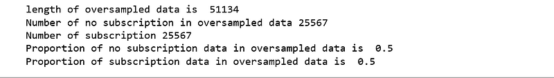

Now we have a perfect balanced data! You may have noticed that I over-sampled only on the training data, because by oversampling only on the training data, none of the information in the test data is being used to create synthetic observations, therefore, no information will bleed from test data into the model training.

Recursive Feature Elimination

Recursive Feature Elimination (RFE) is based on the idea to repeatedly construct a model and choose either the best or worst performing feature, setting the feature aside and then repeating the process with the rest of the features. This process is applied until all features in the dataset are exhausted. The goal of RFE is to select features by recursively considering smaller and smaller sets of features.

data_final_vars=data_final.columns.values.tolist()
y=['y']
X=[i for i in data_final_vars if i not in y]

from sklearn.feature_selection import RFE
from sklearn.linear_model import LogisticRegression

logreg = LogisticRegression()

rfe = RFE(logreg, 20)
rfe = rfe.fit(os_data_X, os_data_y.values.ravel())
print(rfe.support_)
print(rfe.ranking_)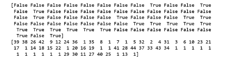

The RFE has helped us select the following features: “euribor3m”, “job_blue-collar”, “job_housemaid”, “marital_unknown”, “education_illiterate”, “default_no”, “default_unknown”, “contact_cellular”, “contact_telephone”, “month_apr”, “month_aug”, “month_dec”, “month_jul”, “month_jun”, “month_mar”, “month_may”, “month_nov”, “month_oct”, “poutcome_failure”, “poutcome_success”.

cols=['euribor3m', 'job_blue-collar', 'job_housemaid', 'marital_unknown', 'education_illiterate', 'default_no', 'default_unknown', 
      'contact_cellular', 'contact_telephone', 'month_apr', 'month_aug', 'month_dec', 'month_jul', 'month_jun', 'month_mar', 
      'month_may', 'month_nov', 'month_oct', "poutcome_failure", "poutcome_success"] 
X=os_data_X[cols]
y=os_data_y['y']

Implementing the model

import statsmodels.api as sm
logit_model=sm.Logit(y,X)
result=logit_model.fit()
print(result.summary2())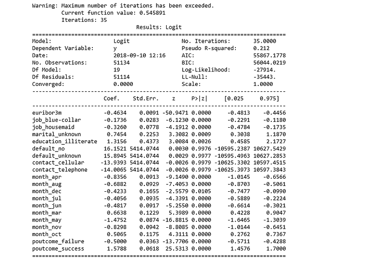

The p-values for most of the variables are smaller than 0.05, except four variables, therefore, we will remove them.

cols=['euribor3m', 'job_blue-collar', 'job_housemaid', 'marital_unknown', 'education_illiterate', 
      'month_apr', 'month_aug', 'month_dec', 'month_jul', 'month_jun', 'month_mar', 
      'month_may', 'month_nov', 'month_oct', "poutcome_failure", "poutcome_success"] 
X=os_data_X[cols]
y=os_data_y['y']

logit_model=sm.Logit(y,X)
result=logit_model.fit()
print(result.summary2())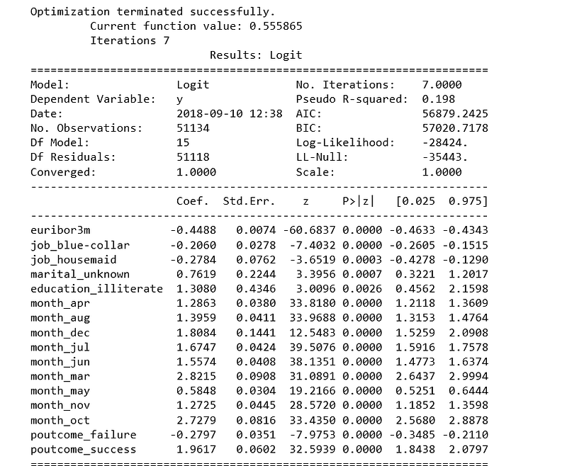

Logistic Regression Model Fitting

from sklearn.linear_model import LogisticRegression
from sklearn import metrics

X_train, X_test, y_train, y_test = train_test_split(X, y, test_size=0.3, random_state=0)
logreg = LogisticRegression()
logreg.fit(X_train, y_train)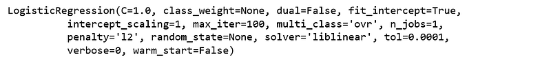

Predicting the test set results and calculating the accuracy

y_pred = logreg.predict(X_test)
print('Accuracy of logistic regression classifier on test set: {:.2f}'.format(logreg.score(X_test, y_test)))

Accuracy of logistic regression classifier on test set: 0.74

Confusion Matrix

from sklearn.metrics import confusion_matrix
confusion_matrix = confusion_matrix(y_test, y_pred)
print(confusion_matrix)

[[6124 1542]

[2505 5170]]

The result is telling us that we have 6124+5170 correct predictions and 2505+1542 incorrect predictions.

Compute precision, recall, F-measure and support

To quote from Scikit Learn:

The precision is the ratio tp / (tp + fp) where tp is the number of true positives and fp the number of false positives. The precision is intuitively the ability of the classifier to not label a sample as positive if it is negative.

The recall is the ratio tp / (tp + fn) where tp is the number of true positives and fn the number of false negatives. The recall is intuitively the ability of the classifier to find all the positive samples.

The F-beta score can be interpreted as a weighted harmonic mean of the precision and recall, where an F-beta score reaches its best value at 1 and worst score at 0.

The F-beta score weights the recall more than the precision by a factor of beta. beta = 1.0 means recall and precision are equally important.

The support is the number of occurrences of each class in y_test.

from sklearn.metrics import classification_report
print(classification_report(y_test, y_pred))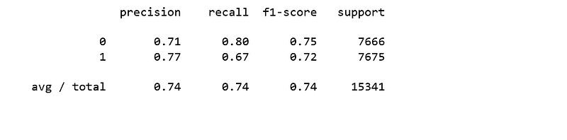

Interpretation: Of the entire test set, 74% of the promoted term deposit were the term deposit that the customers liked. Of the entire test set, 74% of the customer’s preferred term deposits that were promoted.

ROC Curve

from sklearn.metrics import roc_auc_score
from sklearn.metrics import roc_curve
logit_roc_auc = roc_auc_score(y_test, logreg.predict(X_test))
fpr, tpr, thresholds = roc_curve(y_test, logreg.predict_proba(X_test)[:,1])
plt.figure()
plt.plot(fpr, tpr, label='Logistic Regression (area = %0.2f)' % logit_roc_auc)
plt.plot([0, 1], [0, 1],'r--')
plt.xlim([0.0, 1.0])
plt.ylim([0.0, 1.05])
plt.xlabel('False Positive Rate')
plt.ylabel('True Positive Rate')
plt.title('Receiver operating characteristic')
plt.legend(loc="lower right")
plt.savefig('Log_ROC')
plt.show()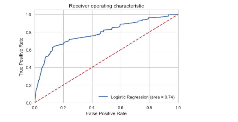

The receiver operating characteristic (ROC) curve is another common tool used with binary classifiers. The dotted line represents the ROC curve of a purely random classifier; a good classifier stays as far away from that line as possible (toward the top-left corner).

The Jupyter notebook used to make this post is available here. I would be pleased to receive feedback or questions on any of the above.

Reference: Learning Predictive Analytics with Python book