Building a Credit Card Fraud Detection Online Training Pipeline with River ML and Apache Flink

In this tutorial, we will go over writing real time python Apache Flink applications to train an online model

In this tutorial the main frameworks that we will use are:

• Flink: a fully distributed real time and batch processing framework
• RiverML: online learning library
• Flask: open source python package used to build RESTful microservices

TL;DR: The code is on GitHub.

Benefits of building an online training pipeline with Apache Flink

Usually we have at least two separate processes when dealing with a ML pipeline. In the first phase we train a new ML model with some data that has been gathered in some amount of time. This is usually called batch training and depending on the quantity of data it can be a slower and more compute intensive process. In the second phase we take the model we produced during the training and we use it on new data to label it, in a process called inference. In more recent years a new paradigm has emerged that is looking to merge training and inference and it’s called online training. Now there are two major benefits from this. Firstly we don’t need that much computation power to do the training and hence the costs are lower, and the ML pipeline is simplified. Secondly an improved ML model, that is trained with more data, is available immediately and in some cases such as fraud detection that is very important because it can reduce the case of false positives and hence detect fraud even faster and better.

Our ML pipeline will have two components: the realtime ingestion part, done using Apache Flink, and the ML serving part using Flask and RiverML, which is responsible for online training. We’ll use Apache Flink to read the data because it’s a low latency and very scalable platform that can be used for big data applications. Initially developed for JVM languages, Apache Flink has now good support for python and that’s what we will use in this tutorial. So let’s get started.

Step 1: setup the python environment for all the dependencies

We’ll use pipenv to install all the python packages that we need in a separate environment. In the github link that I’ve provided there’s a Pipfile that we will use:

[[source]]
url = "https://pypi.org/simple"
verify_ssl = true
name = "pypi"

[packages]
apache-flink = "*"
river = "*"
flask = "*"

[dev-packages]

[requires]
python_version = "3.6"

As you can see we use flink, river and flask with python version 3.6 that is a good option to have all the dependencies compatible to each other.

To install pipenv just run:

pip install --user pipenv

Then in the root of our project we can install all the libraries:

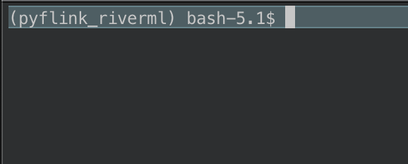
pipenv install

To activate the environment we use the shell command:

pipenv shell

And if everything has run successfully you should see the environment activated like in the next image:

Step 2: create the Apache Flink python consumer

We’ll create a simple python script for this step that will read input credit card transactions and will call the RiverML fraud detection system and the results of the algorithm will be stored in a file. For the input data we will use a dataset that contains transactions made by credit cards in September 2013 by European cardholders. This dataset presents transactions that occurred in two days, where we have 492 frauds out of 284,807 transactions. The dataset is highly unbalanced, the positive class (frauds) account for 0.172% of all transactions. This data is available in the RiverML library.

We create an Apache Flink environment first, which is the entry point for our ingestion app. This is valid for any Apache Flink app that we want to create:

env = StreamExecutionEnvironment.get_execution_environment()
# write all the data to one file
env.set_parallelism(1)

Being a fully distributed framework the processing can be done on multiple threads, but for the scope of this tutorial, we will just use one thread and as a direct result just create one file as the output.

The next thing that we will do is read some of the rows from the credit card data and store them in a list. We will use env.from_collection to to read the list into a Flink DataStream. For the purpose of this tutorial this is good enough, but in a production environment we will probably read this data from an event store such as Apache Kafka or AWS Kinesis and this will ensure we get a continuous stream of records:

# get the credit card data
dataset = datasets.CreditCard()

# create a small collection of items
i = 0
num_of_items = 2000
items = []
for x, y in dataset:
  if i == num_of_items:
    break
  i+=1
  items.append((json.dumps(x), y))

credit_stream = env.from_collection(
        collection=items,
        type_info=Types.ROW([Types.STRING(), Types.STRING()]))

You can also notice that when we create a Flink DataStream we also need to define a schema. In our case we use Types.ROW([Types.STRING(), Types.STRING()]) which represents two strings, the first containing the transaction values and the second one is the label which can be 0 (no fraud) and 1 (fraud). A an example of how the transaction records look like:

'{Time=0.0, V21=-0.018306777944153, V20=0.251412098239705, V23=-0.110473910188767, V22=0.277837575558899, V25=0.128539358273528, V24=0.0669280749146731, V27=0.133558376740387, V26=-0.189114843888824, V1=-1.3598071336738, V2=-0.0727811733098497, V28=-0.0210530534538215, V3=2.53634673796914, V4=1.37815522427443, V5=-0.338320769942518, V6=0.462387777762292, V7=0.239598554061257, V8=0.0986979012610507, V9=0.363786969611213, Amount=149.62, V10=0.0907941719789316, V12=-0.617800855762348, V11=-0.551599533260813, V14=-0.311169353699879, V13=-0.991389847235408, V16=-0.470400525259478, V15=1.46817697209427, V18=0.0257905801985591, V17=0.207971241929242, V19=0.403992960255733}'

Then we use the map method in the DataStream to call the fraud service. Later in the tutorial we will go over creating and starting the microservice, but for now we need to know that the endpoint is http://localhost:9000/predict and the payload that we are sending is {x: feature, y:label} :

# detect fraud in transactions
fraud_data = credit_stream.map(lambda data: \
        json.dumps(requests.post('http://localhost:9000/predict', \
                   json={'x': data[0], 'y': data[1]}).json()),\ 
                   output_type=Types.STRING())

And finally we write the results. We can notice that we use fraud_data.sink_to to write to a file. And the end we also ned to tell Flink that we are ready to execute the pipeline using env.execute() :

# save the results to a file
fraud_data.sink_to(
  sink=FileSink.for_row_format(
            base_path=output_path,
            encoder=Encoder.simple_string_encoder())
        .build())

# submit for execution
env.execute()

The file should contain the ROCAUC metric and the result, false meaning no fraud has been detected:

{"performance": {"ROCAUC": 0.4934945788156797}, "result": false}

Step 3: write the Flask online training microservice

We will compose a standard REST service that will wrap the ML fraud model. This practice is done usually to have the algorithm loosely coupled from the ingestion layer. If we need to deploy another version of the model, we just need to update the microservice with no interference to the Flink consumer.

Initially we create a class that will contain all the ML objects that we will use to interact with the new data that’s being sent to the service. The model is composed from a standard scaler that transforms the data to have zero mean and unit variance and a logistic regression classifier that is a good choice for a binary task such as detecting fraud. We also use the ROCAUC metric to determine how well the algorithm does at the current iteration.

class RiverML:
    # fraud detection model
    model = compose.Pipeline(
        preprocessing.StandardScaler(),
        linear_model.LogisticRegression()
    )

    # ROCAUC metric to score the model as it trains
    metric = metrics.ROCAUC()
fraud_model = RiverML()

Next we actually write the predict endpoint. It will be a POST because we need to retrieve data from the user. There are a couple of important steps here. The fraud_model.model.predict_one(x_data) will make a prediction on the new transaction. As we will see later the initial predictions will not be very good, but as more and more data is being feed into the model, it will give better results. Then we use fraud_model.metric.update(y_data, y_pred) to calculate the ROCAUC metric and fraud_model.model.learn_one(x_data, y_data) to update the model with the correct label. As you can see prediction and learning are done in just one single app.

@app.route('/predict', methods=['POST'])
def predict():
    # convert into dict
    request_data = request.get_json()
    x_data = json.loads(request_data['x'])
    y_data = json.loads(request_data['y'])

    # do the prediction and score it
    y_pred = fraud_model.model.predict_one(x_data)
    metric = fraud_model.metric.update(y_data, y_pred)

    # update the model
    model = fraud_model.model.learn_one(x_data, y_data)

    return jsonify({'result': y_pred, 'performance': {'ROCAUC': fraud_model.metric.get()}})

And at the end we send back a JSON containing the actual prediction and how well the model has performed.

Step 4: running it all

To run the ML pipeline that we’ve just wrote first we need to run the flask app. To do so in a separate terminal run:

python fraud_river_ml.py

And you should get something similar to the following image, flask telling us that the service is available:

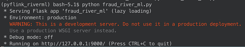
Now we can also run the Apache Flink consumer in a separate terminal window:

python flink_consumer.py --output data

This python script will use the --output parameter to define where we store the results. It should take a minute or so, but after that the script will finish running we should find a file in our location. Again please note that in a production environment the flink consumer script should never stop running as it consumes unbounded data.

If we look in the output file we will see how the model evolves over time. The first iterations will have ROCAUC -0.0:

{"performance": {"ROCAUC": -0.0}, "result": false}
{"performance": {"ROCAUC": -0.0}, "result": false}
{"performance": {"ROCAUC": -0.0}, "result": true}
{"performance": {"ROCAUC": -0.0}, "result": false}
{"performance": {"ROCAUC": -0.0}, "result": true}
{"performance": {"ROCAUC": -0.0}, "result": false}
{"performance": {"ROCAUC": -0.0}, "result": false}
{"performance": {"ROCAUC": -0.0}, "result": false}
{"performance": {"ROCAUC": -0.0}, "result": false}
{"performance": {"ROCAUC": -0.0}, "result": false}

But as we feed more and more data into the logistic regression algorithms this will improve:

{"performance": {"ROCAUC": 0.4992462311557789}, "result": false}
{"performance": {"ROCAUC": 0.4992466097438473}, "result": false}
{"performance": {"ROCAUC": 0.4992469879518072}, "result": false}
{"performance": {"ROCAUC": 0.4992473657802308}, "result": false}
{"performance": {"ROCAUC": 0.49924774322968907}, "result": false}
{"performance": {"ROCAUC": 0.4992481203007519}, "result": false}
{"performance": {"ROCAUC": 0.499248496993988}, "result": false}
{"performance": {"ROCAUC": 0.4992488733099649}, "result": false}
{"performance": {"ROCAUC": 0.49924924924924924}, "result": false}

That’s it! I hope you enjoyed this tutorial and find it useful! We saw how we can write python apps with Apache Flink and train an online classifier with River ML and reduce costs by combining the training and inference layers. This is the backbone of reliable and scalable big data ML applications that we can deploy in production in one of the many cloud providers that offer scalable infrastructure such as AWS, GCP or Azure.