
Build Your Own GraphQL GenBank in AWS
The size of a scientific study: GB of raw data, gets turned into MB of Excel tables, probably written into KB of a manuscript and certainly abstracted into a few Bytes of sentences.
-Sixing Huang
In 2019, I worked in a project commissioned by the Convention on Biological Diversity (CBD) on digital sequence information (DSI) in public and private databases. During the data gathering phase, I needed to download both the GenBank and Whole Genome Seqeuncing (WGS) from NCBI. Those were four TB worth of compressed data in GBK format. GBK is an all-in-one format used widely in bioinformatics. It contains both the metadata and sequences. The irony was, I only needed the metadata, that is, a few GB uncompressed out of those TB compressed data.
That is without a doubt a huge waste of bandwidth, electricity and time. I thought about E-utilities — NCBI’s REST API that was first created in 2008 and has changed little ever since. But REST still would not have got me out of the quandary that is the overdelivery of data from the host. Plus, E-utility only allows three requests per second. At that time due to time pressure, I swallowed my pride and settled on the GBK download. We eventually finished the project and published a report for CBD. But I still have a bitter taste in my mouth and have thought about a way of improvement. One day, I stumbled upon this video:
GraphQL is exactly the interaction that I have always wanted but never gotten from NCBI. The client can tell the server which fields are exactly needed. No more unsolicited data, that is good for the bandwidth and for the environment. Plus, the returned data is in standard JSON format, I can get rid of all those parsers for CSV, GBK, GFF3, FASTQ and FASTA.
Since NCBI does not have GraphQL, I thought that it must be a hard technique. After a day or two doing free tutorials online, it seems that the exact opposite is true: GraphQL is easy to set up, easy to use and language agnostic. In fact, I can show you all the steps in just this one tutorial.
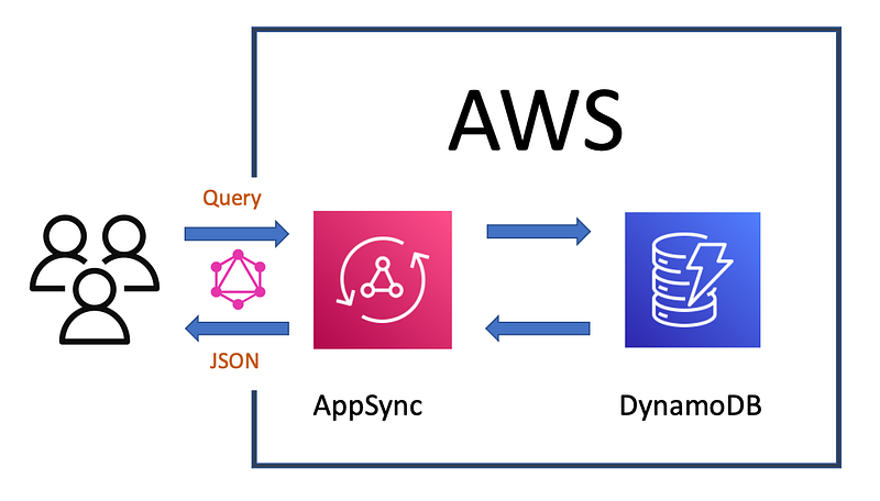
I choose Amazon Web Services (AWS) — DynamoDB and AppSync to be exact. Since this is a small tutorial, I will just use three GBK files. I will import them into a DynamoDB table and set up AppSync as the GraphQL interface. The data will be read only. Finally, I will query it in a Python script. The data and code for this tutorial is hosted on my Github repository:
https://github.com/dgg32/graphql_genbank.
1. Get some GBK data
First, get the GBK files (accession numbers: AB252225, FJ157956, FJ157976) by git clone my repo or from NCBI. In fact, you can use other GBK files. This tutorial tries to demonstrate the metadata fetching ability of GraphQL, so GBK files with the following features are the best: country, lat_lon, db_xref and isolation_source. It is OK that some fields are missing in some of the files though.
2. Set up DynamoDB
Now head over to AWS, choose your region, select DynamoDB and click “Create Table”. Enter “genbank” as “Table Name” and “accession” (keep it as “String”) as “Primary key”. Finish with “Create”.
Once the “genbank” table is online, it is time to use my “gbk_to_dynamodb.py” to import the GBK files into the table. In case you name your DynamoDB table differently, change it in line 9 in the script. You also need to configure your Boto3 credentials beforehand, best with AWS CLI. Then CD into the repo folder and issue the following commands to upload the data:
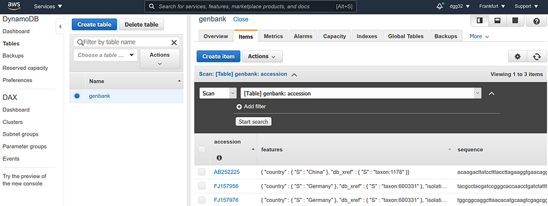
Afterwards, go to DynamoDB and check under “Items” whether the three documents are imported successfully. As you can see, I have structured a GenBank sequence into three columns: accession, features and sequence. The accession is the primary ID. The “features” contains four metadata fields: country, lat_lon, db_xref and isolation_source. And the sequence contains the bulk of data: the sequence.
3. Set up AppSync
Now switch to AppSync. Click “Create API” -> “Build from scratch” -> “Start” and name the API “genbank_graphql”. Once the API is created, click into it and select “Schema” on the left panel. Copy and paste the following schema definition into “Schema” field:
In it, the “schema” block declares what types our GenBank API can do. GraphQL allows three: “query”, “mutation” and “subscription”. In our case, we serve our data in read-only mode so only query is allowed.
The “type Sequence” block models a row in our DynamoDB. As you can see, the three keys here correspond to the columns in our DynamoDB. Similarily, “type Features” just further models the “features” fields. “PaginatedSequences” encapsulates a bundle of sequences plus a nextToken for the next page.
Then comes the “type Query” block. There I have defined three queries. The “getSequencesByCountry” will fetch sequences by country. By the same token, “getAllSequences” will return all the sequences in the database. The last one “getSequence” is used to get a single sequence by a given accession number.
Afterwards, we need to tell AWS what these queries do exactly by implementing their resolvers. A resolver consists of a data source, the action and the response. They can be edited on the right panel by clicking the “Attach” button. Here are the three resolver configurations.
- Click “Attach” next to “getSequence(…): Sequence”, it will open up the “Edit Resolver” page. Choose “genbank_dynamodb” in the “Data source name” drop-down. AWS prepopulates both “request mapping template” (the action) and “response mapping template” (the response) for us and they are the exact codes needed. Click “Save Resolver” to finish.
- Next, click “Attach” next to “getAllSequences”, copy and paste the following code into “request” and “response” fields correspondingly. Don’t forget to save by clicking “Save Resolver”.
3. For “getSequencesByCountry” we need to copy and paste the following code:
That is it. All three GraphQL queries are now configured. Now AppSync is ready to respond to our secure HTTPS request.
If the text above confused you, I can assure you that it is way simpler than it sounds. Readers who want to know the nuts and bolts should have a walkthrough in this AWS tutorial.
4. Test
We can now go for a test drive and get a taste of the power of GraphQL. Click “Queries” on the left panel. Copy and paste the following four test queries into the central panel.
- The first query uses “getSequence” to retrieve the sequence, accession and isolation_source for FJ157956.
- The second query get all the sequences, five per page. But we only want the accession and country fields. No sequences please. In the end, we get the nextToken in case there are more records.
- The third query get sequences from Germany, one scan per page. This time we want the accession, country and lat_lon. In the end, we may get one document and the nextToken in case there are more documents. Copy this “nextToken”. A very confusing fact is that “count” is the number of documents scanned per query, not of documents returned. So if you import AB252225 (from China) first, it will return an empty sequence and nextToken. Only with the next query you will start to see the German sequence.
- The fourth query is actually the “next-page” query of the third query. Replace the nextToken content with the one you just copied in Step 3. This query will return the second German document.
Run these four queries by clicking the orange triangle button. Select the test case one by one and make sure all of them return results successfully.
5. Demo Client
After the tests, let’s build a small Python app that interacts with our API over the internet. I have written the config.py and query.py for this purpose. The first one stores the AWS config data and the latter is the main script. In fact, it simply runs the second query in our test. But first, we need to set the endpoint and the api key in config.py. Click “Settings” on the left panel.
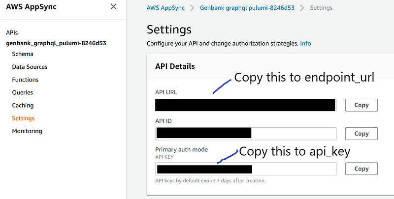
Copy the “API URL” and paste it to “endpoint_url” and “API ID” to “api_key” in config.py. Save the file. Now run query.py by issuing:
python query.py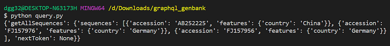
If you see the output of all our sequences like the screenshot above, you are golden!
Conclusion
That is it. We now have a functional GraphQL API serving our nano GenBank. This service is serverless. As to the cost, you can choose flexibly between the on-demand and the provisioned pricing model. It took minimal of work to set up. It is language agnostic and scalable. The main advantage is, it allows users to tailor their requests and get the exact pieces of data. That in turn means a huge reduction in download time and a meaningful boost in productivity. What’s not to love? Imagine if NCBI had this set up, how much time and energy I would have saved a year ago. Now multiply that by a thousand for all the biomedical researchers around the world.
This tutorial is by no mean an in-depth GraphQL tutorial. It does not touch the other two operation types: mutation and subscription. Also it does not explain the inner working of the configurations. Also there are multiple other options to set up GraphQL outside AWS. Finally, iOS and Android integrations have not been mentioned at all.
The same goes for DynamoDB, which deserves its own books. To give GBK users an easier time, I made our DynamoDB schema a simple 1:1 reflection of the GBK file structure. It puts country, lat_lon and so on under the “features” column, just as a GBK file does. As a result, the getSequencesByCountry needs to invoke the “scan” operation instead of “query”. And “scan” costs more in DynamoDB. Therefore, it is better to upgrade these fields into their own columns. Finally, keys and indices should be well desigend for effective partitioning and fast retrieval.
So, it is time to use more GraphQL in our scientific research!
Update: in my new article “Five Commands Build Two NCBI APIs on the Cloud via Pulumi”, I coded the infrastructure with the help of Pulumi. Now just two commands are needed for the setup.


