Hands-on Tutorials

Build your first Graph Neural Network model to predict traffic speed in 20 minutes

A step-by-step coding practice

Graph neural network (GNN) is an active frontier of deep learning, with a lot of applications, e.g., traffic speed/time prediction and recommendation system. In this blog, we will build our first GNN model to predict travel speed. We will run a spatio-temporal GNN model with example code from dgl library.

Spatio-temporal GNN model

We will train a GNN model proposed in this paper published at IJCAI’18: Spatio-temporal Graph Convolutional Networks: A Deep Learning Framework for Traffic Forecasting.

The general idea of this paper is to use the historical speed data to predict the speed at a future time step.

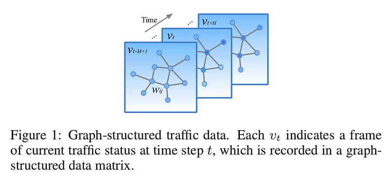
See Figure 1. Each node represents a sensor station recording the traffic speed. An edge connecting two nodes means these two sensor stations are connected on the road. The geographic diagram representing traffic speed of a region changes over time. Our task is to use the historical data, e.g., from v_{t-M+1} to v_{t}, to predict the speed at a future time step, e.g., v_{t+H}. Here M means the previous M traffic observations (v_{t-M+1}, … , v_{t}), and H means the next H time steps, e.g., in the next 30 minutes.

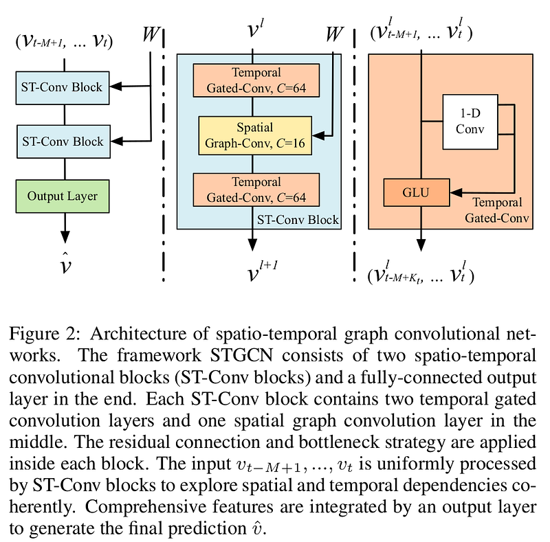
The model consists of a stack of ST-Conv blocks and an output layer. Each ST-Conv block consists of two temporal gated-conv layer and a spatial graph-conv layer in between. The output layer consists of conv, norm, conv, and a fully conv layer.

Prepare the METR_LA dataset

Let’s first prepare the dataset, and then I will explain it next.

mkdir <your working directory>
cd <your working directory>
# clone dgl source code
git clone [email protected]:dmlc/dgl.git
# clone DCRNN_PyTorch repo, because we need the data folder from it
git clone [email protected]:chnsh/DCRNN_PyTorch.git
# copy the data folder from DCRNN_PyTorch repo to dgl repo 
cp -r DCRNN_PyTorch/data dgl/examples/pytorch/stgcn_wave/
# go to the stgcn_wave folder
cd dgl/examples/pytorch/stgcn_wave/

Then download the file metr-la.h5 from this Google drive, and place it in the folder of data. In the end, your directory structure should be like this:

.
├── data
│   ├── metr-la.h5
│   └── sensor_graph
│       ├── distances_la_2012.csv
│       ├── graph_sensor_ids.txt
├── load_data.py
├── main.py
├── model.py
├── README.md
├── sensors2graph.py
└── utils.py

Note that, in the data folder, we need only the files of metr-la.h5, graph_sensor_ids.txt, and distances_la_2012.csv. The other files in the data folder do not matter.

METR-LA traffic dataset is widely used for traffic speed prediction. It contains traffic information collected from loop detectors in the highway of Los Angeles County. 207 sensors were selected, and the dataset contains 4 months of data collected ranging from Mar 1st 2012 to Jun 30th 2012.

The file graph_sensor_ids.txt cotains ids of sensors. The file distances_la_2012.csv contains distances between sensors. These two files are used to create an adjacency matrix, which in turn is used to create a graph using dgl library.

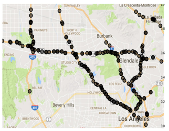
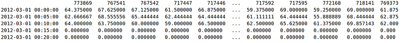
The file metr-la.h5 contains an array of shape [34272, 207], where 34272 is total number of time steps, and 207 is number of sensors. The array contains only speed data, meaning that the GNN model uses the historical speed to predict future speed. No other features (road type, weather, holidays) are involved. The speed was recorded every 5 mins with sensors. The 207 sensors are distributed on roads within the area. See the picture above for the distribution. Speed was collected every 5 mins. So one day should have 24*(60/5)=288 records. So the data of one day is simply an array of shape [288, 207], where 288 is total time steps, and 207 is number of sensors. Since the data was collected across 4 months, there are a total number of 34272 time steps after optional data cleaning. Here below is the first 5 rows. The headers are ids of sensors and the values of content are speed.

To adapt the data for machine learning, we need to prepare features X and target Y. For each sample (time step t), the features X is its speed history of the past 144 time steps from t-144 through t-1 (12 hours). Supposing we have N samples, the shape of X is [N, 144, 207]. The target Y is the speed at a future time step, say t+4, so the shape of Y is [N, 1, 207]. Now that we have (X, Y) pairs, we can feed them to ML.

Train, validate, and test

Now we are ready to train, validate, and test.

First, create a virtual environment and install packages. You need to visit this link to select your right dgl package.

conda create -n stgcn_wave python=3.6
conda activate stgcn_wave
pip install dgl-cu102 -f https://data.dgl.ai/wheels/repo.html
pip install torch
pip install pandas
pip install sklearn
pip install tables

Then we can run main.py by

# maybe you need to adapt your batch size to suit your GPU memory
python main.py --batch_size 10

The main.py does training, validation, and testing in one go. It uses pytorch as an ML framework. In total, it costs nearly one day with a NVIDIA GeForce GTX 1080 graphic card.

As a common way to evaluate travel speed prediction models, Mean Absolute Error (MAE), Mean Absolute Percentage Error (MAPE), and Root Mean Square Error (RMSE) are used in the script. Here below is the end of my log:

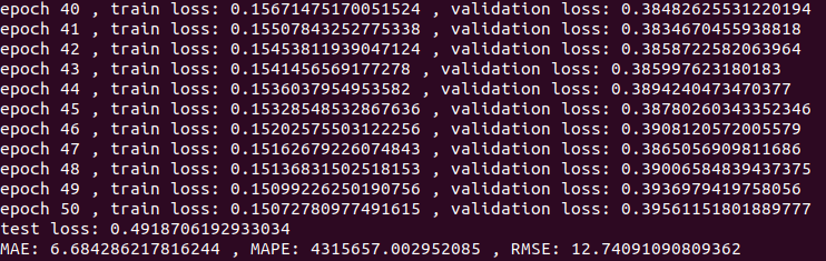
The MAE (6.68) is close to the one (~5.76) claimed in the ReadMe of dgl repository. If I were able to run with default batch size (50), probably I could get even closer result.

References:

[1] Bing Yu, Haoteng Yin, Zhanxing Zhu, Spatio-Temporal Graph Convolutional Networks: A Deep Learning Framework for Traffic Forecasting, 2018, IJCAI.

[2] Yaguang Li, Rose Yu, Cyrus Shahabi, Yan Liu, Diffusion Convolutional Recurrent Neural Network: Data-Driven Traffic Forecasting, 2018, ICLR.