Building a Neural Network to Manage a Stock Portfolio

Introduction to Financial Deep Learning

Introduction

I wanted to write a follow-up article to Build an AI Stock Trading Bot for Free, which describes the development and deployment of an AI model to make trading decisions. This article is to be a precursor to my previous article and introduce deep learning, the mathematics behind it, and a financial application. In my previous article, I emphasize the importance of understanding your AI model beyond importing a library to determine how, and if your network can solve the problem at hand or if there is a more efficient/effective structure. I encourage you to read through this article analytically, the more math pertaining to neural networks you comprehend the better you will be at creating solutions implementing deep learning.

Deep Learning

Deep learning is a subset of machine learning which uses artificial neural networks to learn non-linear relationships from data. Artificial neural networks were inspired by the way our actual brain functions, as we receive data through our senses we process the information and create a response. This idea is maintained in artificial neural networks, data is passed into the neural network and through a series of matrix computations, it yields a response.

It is crucial to note that for this case we will be associating our input data with previously observed outputs we will call the true-y vector. At each layer in the neural network, we will find a preceding weight matrix and activation function. Depending on the structure of the neural network (recurrent, convolutional, etc…) we may even find different computations to better form the desired response. The response is then evaluated by a loss function (performance metric) to determine its effectiveness on unseen data.

Initially, the network’s response is not good in terms of any loss function, meaning the network has to learn how to increase its performance at the task. Fortunately due to the fact that the network is a series of matrix computations we can write it as a composite function with the weight matrices as inputs. The purpose of writing the neural network as a composite function is due to the fact that we can differentiate, more specifically, partially differentiate the neural network with respect to the weights to find the gradient vector of the loss function.

The gradient vector is the collection of partial derivatives with respect to each input (weight matrices) of the function that points in the direction of greatest increase. Once the gradient vector is computed we can step negative that direction to minimize the loss function increasing the neural network’s performance. This is the bare bones version of how we can develop a mathematical function that is capable of learning.

Mathematics of Deep Learning

I will now illustrate the concept of deep learning mathematically. Consider the following structure of the sequential neural network below where data and response are both vectors. (Note: data and response may both be matrices depending on the number of independent/dependent variables, but the same principals follow)

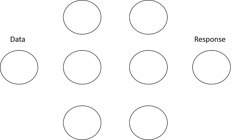
The is an abstraction of the actual mathematics taking place, but we will get to the function definition of this neural network shortly. Consider weight matrices in between each node of the neural network, transforming the input vectors to match the dimensions of the respective nodes.

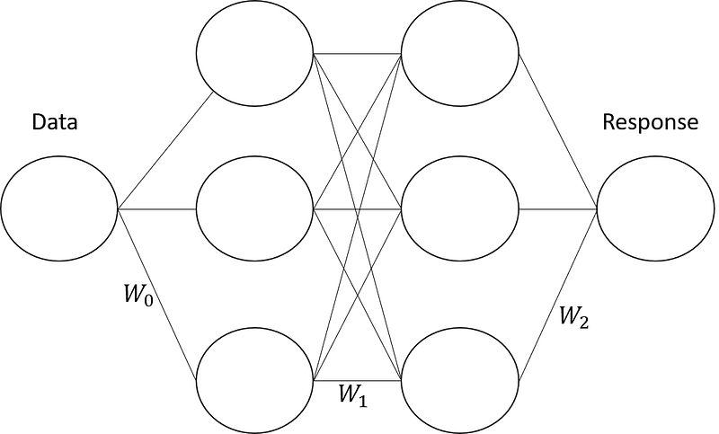
In linear algebra when multiplying matrices we aim to match the inner dimensions to create a new matrix. Consider our input vector, Nx1, to match the three nodes in the first hidden layer we need to multiply it by a weight matrix of dimensions 1x, which looks like (Nx1)(1x3)=Nx3. The inner dimension match and the resulting product creates a new matrix of Nx3 dimensions. This concept goes for each hidden layer with dim(W0)=1x3, dim(W1)=3x3, dim(W2)=3x1, and a response vector of Nx1. The dimensions of the response vector perfectly match the dimensions of the true-y vector, this allows us to compute an error between what was predicted by the matrix computations and what was actually observed.

However, before we start to compute an error based on the randomly instantiated weight matrices we need a function to identify non-linear relationships in our data. This is called an activation function, the activation function we will use for this example is hyperbolic tangent, as I had laid out in my previous article its range is (-1, 1) allowing us to receive an output after rounding of (-1,0,1)(which we may use as a signal to sell, hold, or buy in trading).

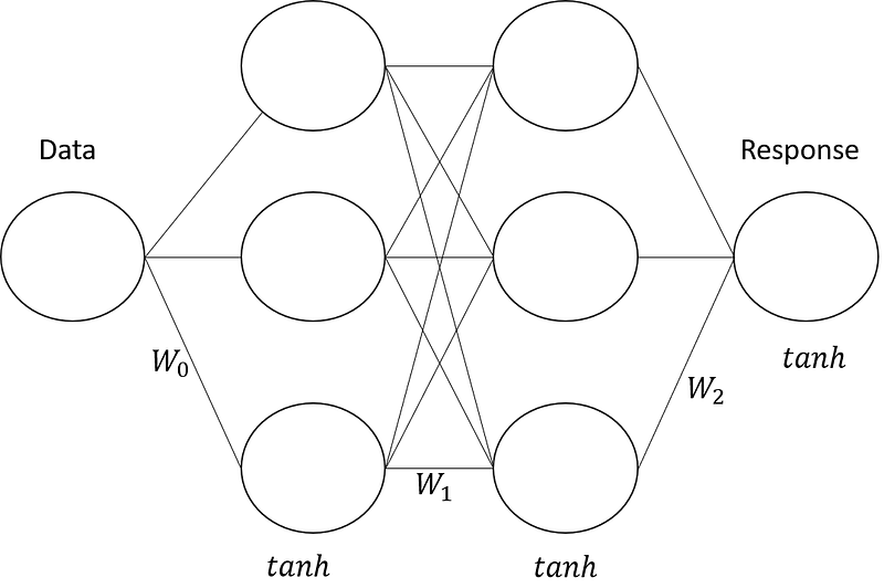
This is the entirety of our sequential model using a picture to abstract the mathematical function that resides therein. Taking the Data that we know is a constant vector of observations, in combination with all of the weight matrices, and the function of a hyperbolic tangent, we can comprise all of these components into one composite function describing the neural network.

Why is this helpful? First off we are removing the abstract diagram and describing the predictive model in terms of a function. The beauty of this solution is that it is continuous and differentiable. This means we are able to optimize this function. However, optimizing this function doesn’t help us, we don’t want to minimize or maximize the function giving us our response vector, we want to minimize the error that is returned from this function. To do that we can actually create another composite function with an output that would be productive to minimize using our true-y vector, a loss function.

This function is directly associated with the performance of the neural network, specifically, this is a function of error in our model. Since it is again both continuous and differentiable we can minimize it, minimizing the error of our model. To minimize the error we will compute the gradient of the loss function and step-less the gradient in each weight matrix for each pass of data through the model. This will allow us to update the weights and step in the direction of the greatest decrease.

This is how the neural network learns. Every time the data is passed through the function for the neural network it computes a predicted-y, this is then compared against the true-y to compute a loss. Then using the gradient vector we update the weights to move in the direction of greatest increase (less the gradient vector to each weight matrix respectively) until a relative or global minimum is reached. It is critical to note that this is why we break out model into training and testing sets, otherwise, the loss function will be minimized by forcing the weights to values that best fit all observed data, not to what generalizes best. These are the key concepts behind essentially every type of neural network, though the dimensions of the input, output, intermediate function computations, etc… may change the idea of passing data through that iterating back to minimize an error stands prevalent in all deep learning models.

Financial Deep Learning

Now that we understand how a basic sequential model functions we can implement it in a practical real-world investing problem. Often times we have an optimal, diversified portfolio, (maybe created by using my pipeline) and we want to manage the portfolio according to a predetermined set of rules. Instead of building an algorithmic trading system with investment management based on control we can build a neural network to act on our portfolio by training it on certain instructions. In this article, we will be using Python and its accompanying libraries to build this neural network. To give you an idea of how this can be implemented, consider a diversified portfolio in which we wish to mitigate systemic risk. We can train a neural network to liquidate a portfolio if it declines by x% any given day acting like a personal circuit breaker. Obviously, that condition is arbitrary and the model can be trained to follow any annotated signal you specify.

Building the Dataset

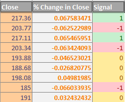
To create the dataset you need a vector of your portfolio value over a consistent discrete time interval. If you don’t have access to that data for your portfolio you may also use the historical data associated with the assets in your portfolio over the same time interval to accomplish the same thing. In this case, consider my ‘diversified portfolio’ consisting of one share of TSLA. I download the historical data from Yahoo! Finance using a discrete-time interval of one week between closing prices. I create a new column that computes the % change in equity price over the week, and a column that follows the conditions I specified for buy/sell/hold.

Building the Neural Network

Now comes the interesting part, building the neural network. We already know how neural networks function, the wide variety of programming libraries available to us makes the implementation very easy. There are a lot of questions that need to be answered based on our understanding of neural networks: type, structure, activation, loss… For the purpose of this article, we will be using a sequential model, standard dense layers, hyperbolic tangent activation function, and a hinge loss. If you are interested in learning how to pick each component to solve the problem at hand you can see this fantastic book by François Chollet, or to learn why we chose the structure for this portfolio management problem, see my other article. Fortunately, the code is very straightforward…

Just like that, you now have an AI model capable of buying and selling based on the conditions set forth by your dataset…

Conclusion

The concept of training an AI with data annotated to a specific rule-set seems counterproductive. Why not just embed the rule-set directly into the algorithmic trading system? The optimal way to implement this technology isn’t to follow a discrete set of rules but rather a continuous set of rules constantly being updated by a combination of reinforcement, unsupervised, and online supervised learning algorithms. Reinforcement learning is learning without a predetermined set of rules but a fitness function and optimizes similarly to a genetic algorithm. Supervised learning is the model equivalent to the AI portfolio manager we just built. Finally, unsupervised learning is used to identify unknown relationships in data. In later articles, I will detail the use of reinforcement learning which is, in my opinion, the most productive method for financial solutions. Reinforcement learning offers financial solutions including but obviously not limited to building trading models, managing portfolios, hedging with derivatives, etc…