DATA STORIES | SPORT ANALYTICS | KNIME ANALYTICS PLATFORM

Boost your Passion for Sport! Analyze your Sports Data with KNIME + Strava

Discover and visualize your sport feats without the need to be a programmer. Prepare to be amazed!

Passion for sport and technology come together in this exciting guide, where we’ll explore how to harness the power of KNIME to analyze Strava geospatial data. If you are a sports enthusiast and want to discover new perspectives on your activities, you have come to the right place! We’ll learn how to perform a detailed data analysis step-by-step, from downloading Strava data to viewing routes on a map.

You can download the workflow for free from the KNIME Community Hub.

Step 1: Download geospatial data from Strava

We are going to obtain the data from Strava, but it could be from any other platform. In our case, we chose the GPX format to download the data.

Please note that, to get the data, we could have connected via API to Strava directly. We didn’t do it this way to simplify the workflow, but if you are interested in seeing this way of retrieving the dataset, let us know in the comment below and we will make another article where we will connect to and retrieve data directly from Strava. For example, we could have also connected via API to the website of the State Meteorological Agency of Spain and gotten the temperatures or the wind during training… Interesting, isn’t it?

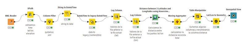
Step 2: Import the data with the XML Reader node

Once we have our data downloaded locally, we use the XML Reader node to import the dataset and start analyzing it.

Step 3: Extract specific data with the XPath node

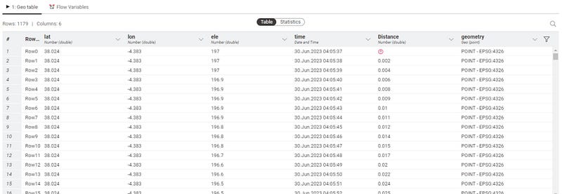
With the help of the XPath node, we select and extract the specific field that we want to analyze. In this case, we extract:

• Spatial coordinates, i.e., latitude and longitude.
• Date and Time.
• Elevation.

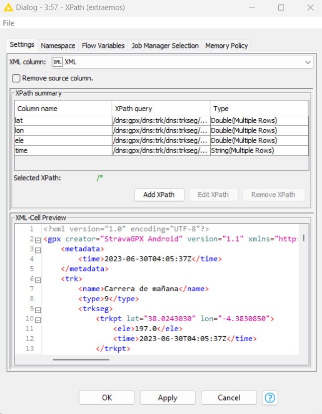
With this minimal set of data, we are ready to build an analytical application. However, we could further enrich our analysis by importing data about the heart rate monitor, power data if we are riding a bike, cadence, etc.

Step 4: Format dates with the String to Date&Time node

Time to make sure our dates are readable and easy to manipulate. We use the String to Date&Time node to convert dates into the proper format and make future operations easier.

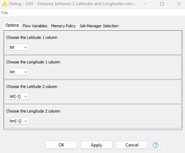
Step 5: Calculate traveled distances with the Lag Column node and distance between 2 lats and lons

The analysis of the distances covered in our sport activities is essential to know our achievements. To do that, we use the Lag Column node and the “Distance Between 2 Latitudes and Longitudes using Haversine formula” component.

First, with the Lag Column node, we create additional columns in our table, where each row contains the geospatial location (latitude and longitude) of the previous activity. This allows us to easily calculate the distances between consecutive locations.

Then, with the “Distance Between 2 Latitudes and Longitudes” component, we take advantage of the Haversine formula to calculate the distance between geographic locations. The formula takes into account the curvature of the Earth, providing precise results for our sports activities.

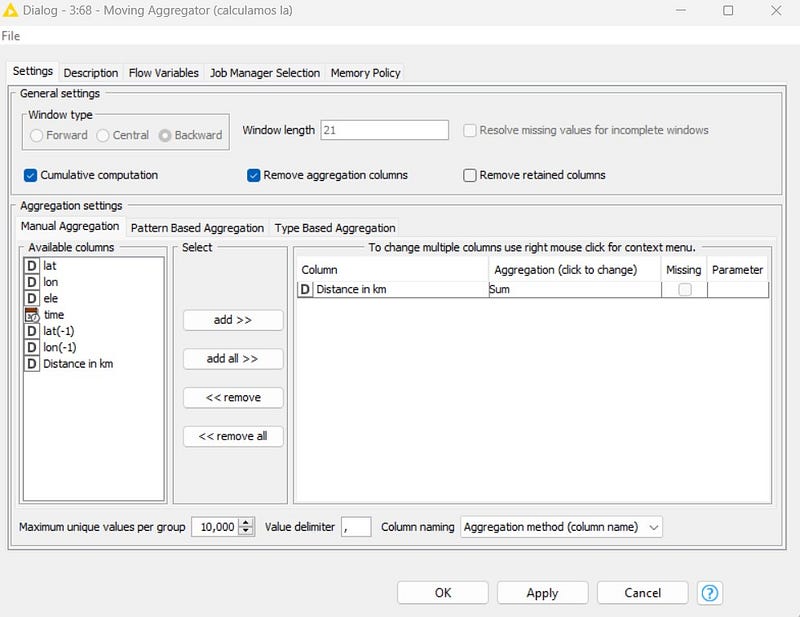
Step 6: Calculate the total distance and clean the table

In this step, we will address two essential tasks: calculating the total distance travelled and cleaning the table for analysis and visualization.

To get a global perspective of our sports activities, we need to calculate the total distance travelled. We use the Moving Aggregator node to sum the distances between geographic locations, previously generated with the “Distance Between 2 Latitudes and Longitudes” component.

Once we have calculated the total distance, it is important to clean up our table and prepare it for analysis and visualization. We use the Table Manipulator node to remove the columns we don’t need and rename the column containing the distance.

Step 7: Transform Latitude and Longitude with the Lat/Lon to Geometry node

Now that our data is ready, it’s time to perform the final transformation before visualizing it. We use the Lat/Lon to Geometry node to convert latitude and longitude coordinates into a geometry format that is more suitable for visualization on an interactive map (see results below).

Step 8: Visualize the data with the KNIME Geospatial View node

The Geospatial View node is a powerful tool that allows us to visualize our geospatial data on an interactive map. With this node, we can explore our routes and sport activities visually and without coding.

In this case, we’ll use elevation as the column to change the colour of the track on the map, but we can adjust both thickness and colour in this node based on many other columns, e.g., speed, heart rate, power, etc.

By customizing the visualization according to different variables, we can obtain a more detailed and meaningful perspective of our sports activities.

Conclusion

Blending KNIME and Strava, we have figured out how to turn our geospatial data into valuable and visually compelling information. From calculating the total distance travelled to preparing and displaying our sporting achievements, KNIME proves its versatility as a powerful tool for analyzing geospatial data without requiring any programming knowledge.

But the potential of KNIME goes much further. Imagine what we could achieve by combining data from our sport activities with information from other sources. Take, for example, weather data, hours of sleep, power in cyclists, speed, heart rate — everything you want. With KNIME, we have at our disposal endless possibilities to enrich our analysis and obtain a complete view of our performance.

So do not wait any longer and try it out yourself! If you want to further explore the KNIME universe and find out how to integrate APIs and perform deep analysis, just say so in the comments. We will be happy to share with you more insights and help you boost your sport performance.

PS: Don’t forget to follow to me on LinkedIn and Twitter to support my work. Or subscribe to my weekly KNIME newsletter in Spanish on LinkedIn.

Thanks for reading!