Boost Confidence In Your Backtesting Results — Two Simple Approaches

Are you confident your average expectancy is positive?

So, you’ve made a trading strategy and decided to backtest the results; you find that your strategy has a positive expectancy on average — awesome, an edge in the market!

But wait, are you sure?!

Market dynamics are incredibly complicated, and honestly, a backtest can never give 100% certainty of the future of strategy outcomes. We’re not clairvoyants unfortunately, but data-driven traders/investors… so put away the crystal ball, it probably won’t help us here (and if it does, please let me in on the secret!).

But can we at least estimate where our expectancy should be? Well, we can certainly take a more rigorous approach here, and instead of just using a mean expectancy, why not throw in some confidence intervals? This may yield a higher degree of statistical certainty on the strategy.

Let me illustrate with a simple example from a set of trade results obtained via average crossover strategy (which I will describe later!).

From 1993: an average of 1.27% per trade (red dashed line)
From 2019-February 2023: an average of 1.88% per trade (black dashed line)

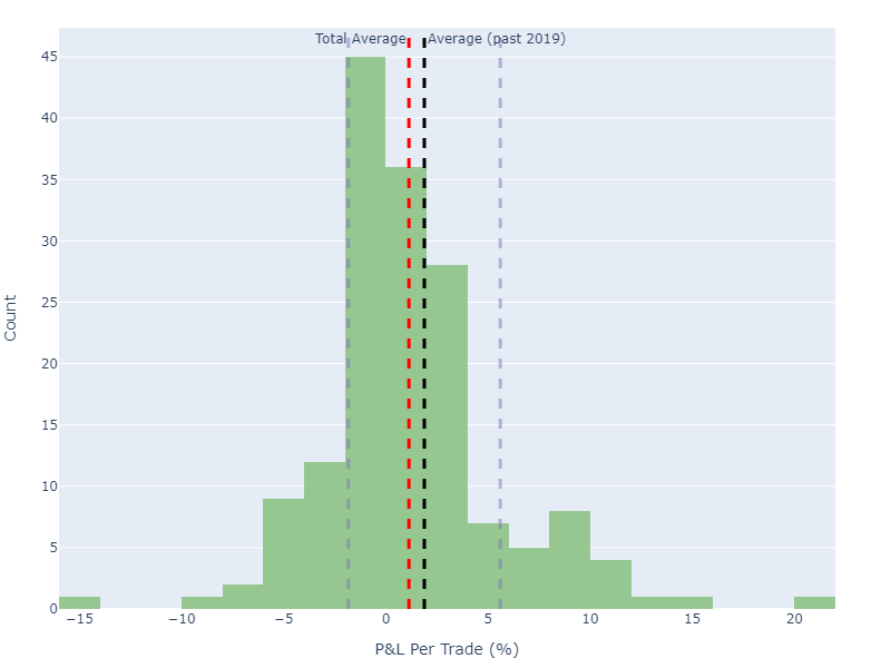
The fainter lines are simple confidence intervals on the 2019–2023 average — this says that the true strategy average lies within these bounds with a 90% confidence; you can see that the red line certainly does lie within these bounds.

However, given the rather small sample of trades since 2019, the confidence bounds are super wide! Would you trade this strategy, given that the lower confidence bound is negative? This shows the power of going slightly further than just calculating an average and being done with your analysis!

Read on, and I’ll show you some ways you can estimate these bounds, and also, some of the things you should be careful of!

The Strategy

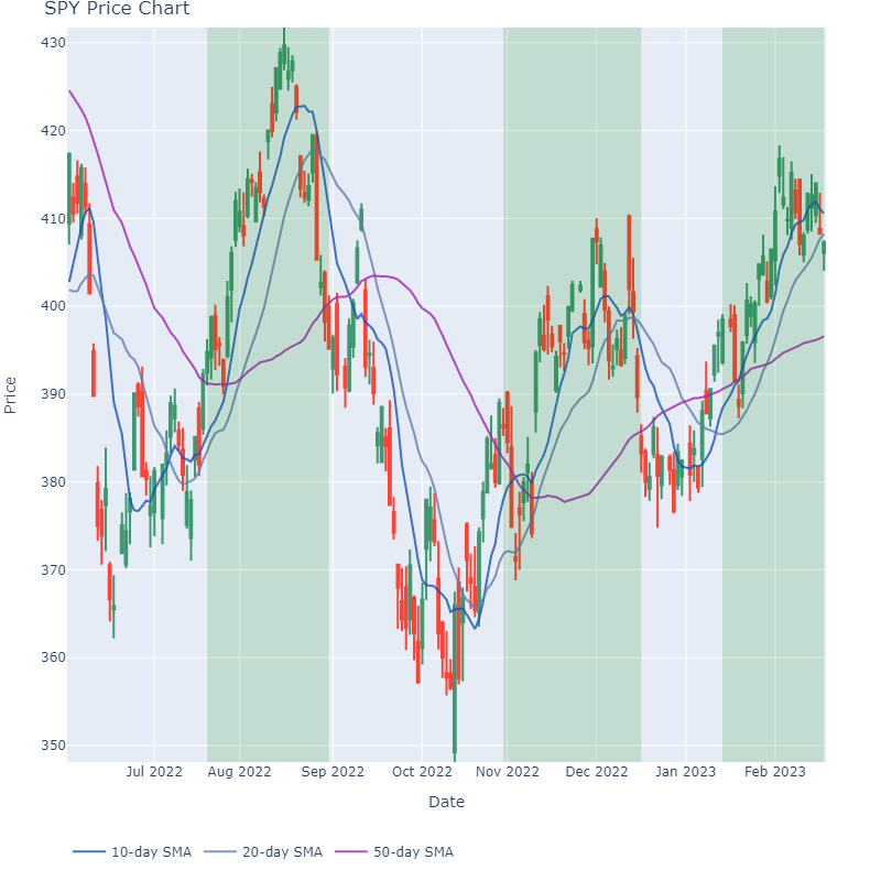
Before we begin, let’s describe the strategy that we’ll be drawing our results from. We are going to trade the SPY only, and enter if the following criteria are met:

The 10 day simple moving average >= 20 day simple moving average.
The closing prices are above the 50-day moving average.

The entry is on the next opening price, and we exit if the 10-day moving average <= 20-day moving average. It’s a simple strategy, and used here purely to show how to analyze the results a little deeper — and not an indication of whether you should trade it!

For you visual learners, here’s an image showing the holding duration for a few trades (highlighted areas):

To run the backtest, please use this code here! This will save a file called “trade_results.csv” which shows the entry, exits, and P&L for each trade.

import numpy as np
import pandas as pd
import yfinance as yf

TICKER = 'SPY'
MOVING_AVERAGES = [
    10, # Fast moving average
    20, # Slow moving average
    50, # Extra signal moving average
]


def perform_backtest(
        close_prices: np.array, 
        open_prices: np.array, 
        fast_ma: np.array,
        slow_ma: np.array,
        signal_ma: np.array,
    ):
    
    # A flag to see if we are in a trade
    holding = False

    # Empty lists to store the outcomes
    bought_on = []
    sold_on = []
    result = []
    
    for day in range(1, close_prices.shape[0]):
        
        if (
                not holding 
                and fast_ma[day-1] >= slow_ma[day-1] 
                and close_prices[day-1] > signal_ma[day-1]
            ):
            
            bought_on.append(day)
            price_bought = open_prices[day]
            
            holding = True

        elif holding and fast_ma[day-1] <= slow_ma[day-1]:
            
            sold_on.append(day)
            result.append(open_prices[day]/price_bought - 1)
            
            holding = False
            
        
    # Close the final trade to get the stats until the latest date
    if holding:
        sold_on.append(day)
        result.append(open_prices[day]/price_bought - 1)
        
    return (
        np.array(bought_on),
        np.array(sold_on),
        np.array(result),
    )


def get_moving_averages(
        df : pd.DataFrame,
        moving_averages: list
    ):
    
    for ma in moving_averages:
        df[f'{ma}_ma'] = df['Close'].rolling(ma).mean()
        
    return df.dropna()


def get_result_df(df: pd.DataFrame):
    
    bought_on, sold_on, result = perform_backtest(
        close_prices = df['Close'].values,
        open_prices = df['Open'].values,
        fast_ma = df[str(MOVING_AVERAGES[0]) + '_ma'].values,
        slow_ma = df[str(MOVING_AVERAGES[1]) + '_ma'].values,
        signal_ma = df[str(MOVING_AVERAGES[2]) + '_ma'].values,
    )
    
    dates = df['Date'].values
    
    results = pd.DataFrame({
        'date_bought': dates[bought_on],
        'date_sold': dates[sold_on],
        'result': 100*result,
    })
    
    return results


if __name__ == '__main__':
    
    df = yf.download(TICKER).reset_index()
    df = get_moving_averages(df, MOVING_AVERAGES)
    
    results = get_result_df(df)
    
    # Print the statistics
    print('Average : ' + str(results['result'].mean()))
    print('Number of Trades : ' + str(results.shape[0]))
    
    # Save the files to csv
    results.to_csv('trade_results.csv')

Please note that this code also downloads the price data from yahoo finance, using the yfinance library; see my guide for more information!

How to Download Free Stock Price Data with Python - From Zero to Hero! - Geekonomics

Are you tired of manually entering stock ticker symbols into your favourite finance website? Well, it's time to say…

geekonomics.co.uk

Approach 1: Simple Confidence Intervals

The absolute simplest way to generate quick-and-dirty confidence intervals is to use the simplistic “z-score” approach, using this formula for the left and right intervals:

Where:

μ is the sample mean
σ is the sample standard deviation
Z is the critical value from the standard normal distribution corresponding to the desired confidence level
n are the number of samples

We can get Z in Python by using the following:

import scipy.stats as st
z = st.norm.ppf(0.9) # Z score for a 90% confidence

For example, in a 90% confidence bound Z = 1.28.

Important note! This type of confidence interval can only be used when you have either a good few samples (at least more than 30) and also when your data appears to be normally distributed.

How do we tell if the data is normally distributed? A quick approach is to plot the data, does it look like it follows a bell-curve shape? There are fancier ways to do this of course, but that’s the fastest!

For example, the plot in the introduction is not 100% normally distributed — I’d argue that it’s right-tailed! So, these confidence intervals may not be entirely appropriate for this distribution of data; but arguably, it’s better to at least analyze these intervals than just considering the average by itself!

Approach 2: Bootstrapping

We have already seen in the introduction that the strategy may perform better or worse at different times, perhaps something in the market changes? Or maybe more people start using that strategy, making it a “self-fulfilling prophecy”?

Bootstrapping is a powerful statistical technique that involves creating many resamples of your original dataset (with replacement) to estimate the distribution of a statistic of interest. By repeatedly resampling from your data, you can simulate many different possible datasets that could have been generated from the same underlying distribution.

Ew, that’s complicated! Why is it important?

It allows us to better estimate strategy performance irrespective of market conditions. Say in one sampling we take 20 trades, 5 may come from 2001, another 5 from 2007, another 5 from 2014, and another 5 from 2022 — these are entirely different years/conditions!

In super simple terms, when we bootstrap we sample n results at random, take an average, store it, randomly sample another n samples, take an average, store it, and repeat m times! This will give us a distribution of sample averages of length m (also we sample with replacement, which means we can sample the same point more than once).

How do I implement the bootstrapping?

Bootstrapping has been made super easy by using the scipy library; just check out this code here (most of it is plotting code!):

import pandas as pd
import numpy as np

from scipy.stats import bootstrap

import plotly.graph_objects as go
from plotly.subplots import make_subplots
import plotly.io as pio
pio.renderers.default='svg'


if __name__ == '__main__':

    df = pd.read_csv('trade_results.csv')
    res = bootstrap(
        data=(df['result'].values, ), 
        statistic=np.mean,
        n_resamples=5000,
        confidence_level=0.95,
    )
    
    print('Average:', np.mean(df['result']))
    print(res.confidence_interval)
    
    fig = make_subplots(
        rows = 2,
        cols = 1,
        shared_xaxes = False,
        vertical_spacing = 0.15,
        subplot_titles = ('Trading Results', 'Bootstrap Histogram'),
        row_width = [0.4, 0.4]
    )
    
    fig.add_trace(
        go.Histogram(x = df['result'], showlegend=False),
        row=1,
        col=1,
    )
    
    fig.add_vline(
        x=df['result'].mean(), 
        line_width=3, 
        line_dash="dash", 
        line_color="red",
    )
    
    fig.add_vline(
        x=res.confidence_interval[0], 
        line_width=3, 
        line_dash="dash", 
        line_color="black",
    )
    
    fig.add_vline(
        x=res.confidence_interval[1], 
        line_width=3, 
        line_dash="dash", 
        line_color="black",
    )
    
    fig.add_trace(
        go.Histogram(x = res.bootstrap_distribution, showlegend=False),
        row=2,
        col=1,
    )
    
    fig.update_layout(
        yaxis1 = {'title': 'Count'},
        yaxis2 = {'title': 'Count'},
        xaxis1 = {'title': 'P&L Per Trade (%)'},
        xaxis2 = {'title': 'Mean P&L (%)'},
        legend = {'x': 0, 'y': -0.1, 'orientation': 'h'},
        margin = {'l': 50, 'r': 50, 'b': 50, 't': 25},
        width = 800,
        height = 600,
    )

    fig.show()

When I ran this, it said that my confidence interval for the average profit/loss was between [0.5%, 1.86%]. Here is the figure that I got:

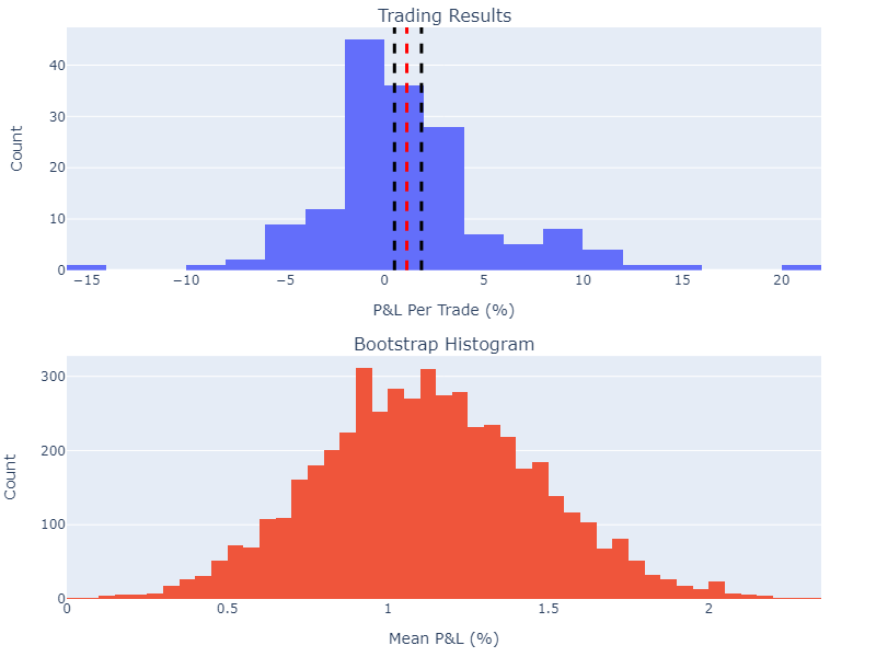
You can see in the above that across all bootstraps, we had a positive expectancy in the strategy (given by the bottom histogram). So you could look at this and reason that in the long term, the strategy will produce a positive expectancy.

The best thing about bootstrapping is that it doesn’t have to be done on the mean P&L — you can choose any statistic! What about the median or standard deviation? Doing such analysis will help you better understand the variability in a strategy performance, much better than some simple statistics will!

But beware! This method assumes that your data must be i.i.d (independent and identically distributed). Over a longer timespan (like this 20-year backtest), it’s more likely that your data will be i.i.d — this may not be true if you limit your backtest to a few months!

Some Final Thoughts

Hopefully, this article has inspired you to dig a little deeper when you obtain a set of backtesting results — it’s very easy to obtain an average result, but harder to fully appreciate the ins and outs. Confidence intervals are a nice way of estimating the variability in your strategy performance, particularly over the long term where we have a variety of market dynamics!

But be very careful how you apply these approaches. If your data is not normally distributed, then you could hit issues with the Z-score approach; likewise, with bootstrapping, if you apply it to just a select few trades over a short period, you run the risk of “overfitting” to certain market conditions (unless that’s your aim, of course!).

If you’re going to listen to one thing from this article, then always put on a critical hat when investigating your results and research fully the methods you are using to be sure you’re not violating any assumptions those methods are based upon!

Until next time — happy analyzing!

Thank you for reading, I hope you enjoyed the article! Please feel free to connect with me on LinkedIn — I’d love to hear from you! Also feel free to follow/DM me on twitter.

If you are thinking of getting a medium account, then please consider supporting me and thousands of other writers by signing up for a membership. For full disclosure, signing up through this link grants me a portion of your membership fee, at no additional cost to you (a win-win for sure!).

Originally published at https://geekonomics.co.uk on February 19, 2023.

Subscribe to DDIntel Here.

Visit our website here: https://www.datadriveninvestor.com

Join our network here: https://datadriveninvestor.com/collaborate