Black Litterman Model: Investment Management with Python and Machine learning Specialization lecture Notes Part-VIII

This week we will cover week 3 of course 2 in the Specialization. For earlier parts, please refer here. This week, we will be covering the Black Litterman portfolio optimization, which is a bayesian algorithm, and we will cover why return-based estimates are not a good idea

EXPECTED RETURNS ARE NOT ROBUST

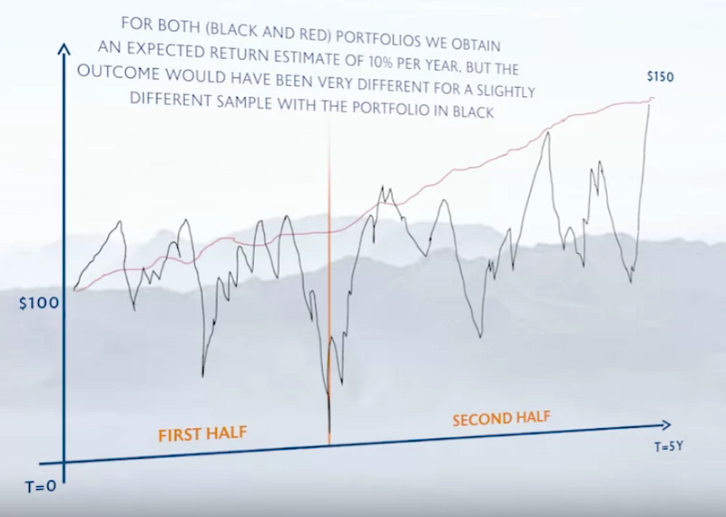
• In the above diagram, we have a black-colored portfolio and a red-colored portfolio. We can see that both portfolios will generate the same return as they end up at the same point. But the black-colored portfolio is more volatile, whereas the red one is less volatile.
• Now, we have divided the total sample period into two halves, then in the first half, we can see a stark difference between the two portfolios. The black one generated negative returns. THUS THE EXPECTED RETURNS ESTIMATES DEPEND ON THE SAMPLE PERIOD.
• So, we cannot use the statistical measure of expected returns, what can we do?

FREQUENTIST VS. BAYESIAN APPROACH

• In the frequentist approach, we have some expected estimates after getting exposed to the data, whereas, in the bayesian approach, we have some prior knowledge about the data.
• For example, A frequentist without seeing the data, cannot say whether it is fair or not. So in 10 tosses, if we get 6H and 4T, then the frequentist will conclude that the coin is not fair and Pr(H) = 0.6. But a bayesian statistician will assume that the coin is fair. Now, after seeing the data it will update the probability based on the Bayes theorem. So 10 tosses are not significant to updating the prior probabilities, but if we have 1000 tosses, then we will be inclined to the conclusion that the coin is not fair
• So the Bayesian approach is more robust compared to the frequentist approach, as the latter is entirely sample dependent. A small change in the sample will lead to a substantial change in the estimates. But the bayesian algorithm is robust to the sample proportion.
• You can employ some shrinkage techniques with the mean. First, find the average mean return for a particular stock (μi). Then find the grand mean or the average of all the stock's mean return (μi’s), called μ. Then shrink the parameters by δμi + (1-δ)μi. This will reduce the variance of the returned estimate.
• Let’s get back to the Bayesian approach now. For a bayesian model, we need a prior. We can’t pick an individual prior for each stock, hence we need to pick a uniform prior or agnostic prior. So we have all the expected returns as equal, as prior.
• As all the expected returns are equal, so the Maximum Sharpe ratio (MSR) portfolio is the Global Minimum variance (GMV) portfolio. We know that the Sharpe ratio is the ratio of expected returns and variance. If the expected returns are the same for all, then optimization is only possible with variance, thus minimizing it, hence a GMV portfolio.

BUT

• This is a bad assumption, we cannot assume that the expected returns for each stock are equal, as all the stocks have a different risk profile. So we need a second kind of agnostic prior.
• So the second agnostic prior is that all the assets will have the same Sharpe ratio

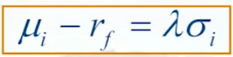
• So for the amount of risk that we are taking, we will get a proportional excess return for the stock so that the Sharpe ratio across the stocks is the same. Hence, the MSR portfolio is the Maximum diversification portfolio, as for each individual asset you are taking proportional risks.

BUT (the second one)

• According to the asset pricing model, only systematic risk is rewarded and any specific risk in a portfolio can be diversified away.
• But when we consider the equal Sharpe ratio portfolio, we are considering all kinds of risks, that is systematic and specific risks. So we need to estimate the expected returns which are proportional only to the systematic risk, as we are assuming that the specific risk can be diversified away.
• So, we can use factor models to distinguish between rewarded and non-rewarded risks.
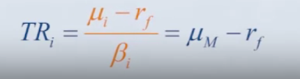
• We will start with the CAPM model as the factor model, so the excess expected return is proportional to the beta of the stock. Or also we can say that instead of the Sharpe ratio is equal for each stock, the Treynor ratio is equal for each stock.

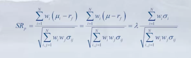
• So maximizing the Sharpe ratio means the following

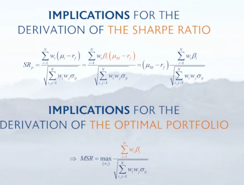
• So as the expected return is proportional to the market excess return, which is the same for all stocks. We can find the MSR portfolio by maximizing the summation in the numerator.
• Selecting the CAPM as a factor model will lead to smaller deviations in the range of the returns. But we should not rely on a single-factor model, as CAPM is not the true asset pricing model. As CAPM cannot describe all the historical returns.
• So for a multi-factor model, we will have the following.

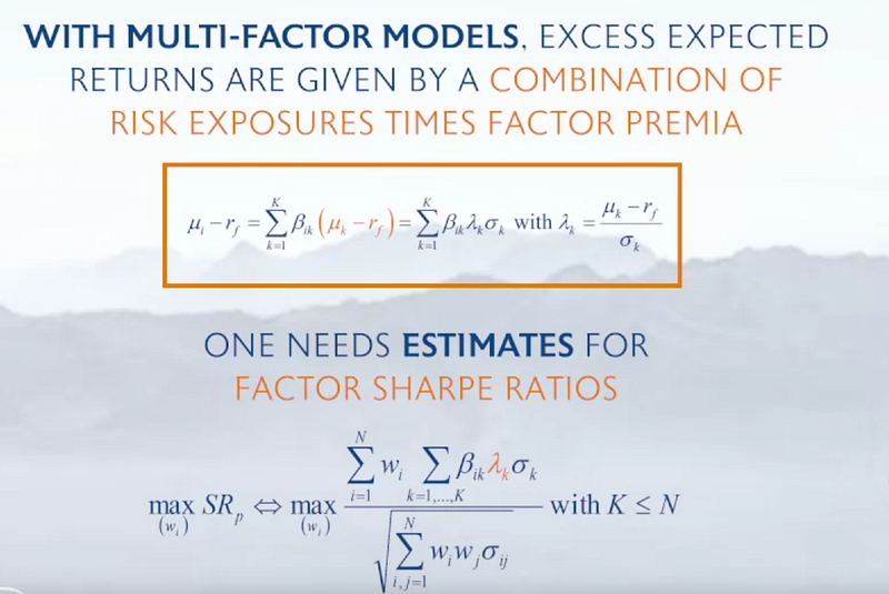
• So, we can see that we need to estimate the shape ratio (λk) for each factor now, which will incur additional estimation errors.
• Let’s check three types of approaches that we can take to this problem

1. Agnostic approach, where we will assume that all the factors have the same Sharpe ratio. This is not necessarily true, but we can assume it
2. Frequentist approach: We can take a long sample and then compute the Sharpe ratio for each factor.
3. Active approach: It is valuable for an active portfolio manager to set forward-looking return estimates or views that can be used as a Sharpe ratio for all the portfolios. So this is used in Black Litterman portfolio optimization.

LET’S GO THROUGH THE ACTIVE APPROACH:

• To measure the performance of an active approach, we need a relevant anchor point or benchmark return. In the Black Litterman (B&L) model, the market portfolio as per CAPM is used as an anchor point.
• The B&L model is an application of bayesian analysis to portfolio construction. For Bayesian analysis, we need the following things: (i)A prior, (ii)A manager view distribution (similar to likelihood), and (iii)A posterior.
• Before going into the B&L model, let’s understand the active views of the Manager.

ACTIVE VIEWS

• A view is like a quantified opinion like Apple will increase by 5%. It is an absolute view. If Apple will increase by 5% relative to Microsoft, then it is a relative view.
• A view is expressed as a normal distribution with a mean equal to Q and a standard deviation given by Ω. So Pπ = Q + ϵ, where ϵ ~ N(0,Ω). Here π is the implied excess return. Also, let K be the total number of views expressed by the Manager (both absolute and relative views). So here P is the KxN matrix that identifies the assets involved in the views. Q is the K-vector of the expected returns on these portfolios. Finally, Ω is a KxN matrix or error terms in the views (confidence levels or the standard deviation).
• If the ϵ term has a higher standard deviation (Ω), then the Bayesian posterior will converge to the benchmark or prior return. So if the manager does not have a lot of confidence in his/her views, then the posterior distribution will converge to prior return weights (like cap-weighted S&P500). So you will always be safeguarded by investing in market-weighted portfolios. Your views will modify the weights to capture your expected returns based on the confidence that you have in the view.

MATHEMATICAL NOTATION FOR THE B&L MODEL

• We will be going through this video, to understand the B&L Model more clearly.
• The video starts with the shortcomings of the Markowitz model, where the weights are concentrated and with small changes in expected return, the weights change a lot due to blind optimization of the minimum variance.
• The B&L reverse optimizes to solve for the excess returns rather than weights. Let’s unravel this, but first, start with the Utility function. U = (weighted average of rewards )— 0.5*(Risk Aversion)*(variance and covariance of the portfolio).

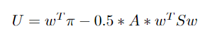
• Here w is the weight vector (the sum of the weight vector is equal to 1), π is the return vector, A is the risk aversion parameter and S is the variance and covariance matrix. The value A is specific to an individual, higher A means that the investor is more risk averse, and his/her utility or happiness will decrease if we take more risk. So if you are taking an equal amount of risk for a risk-averse and a risk-seeking person, then you need to compensate the risk-averse person more. In some papers, the risk aversion is set based on some heuristics like

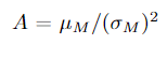
• Here μ is the market return and σ is the market volatility.
• So if you take a first-order derivative with respect to w, then we can find the maximizing objective. Also, if you see that if you take the second derivative with respect to w, you will get -AS, thus it will maximize the utility.

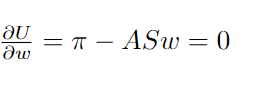
• Now, instead of solving for w, let’s solve for π. Let us take the w to be the cap-weighted market weight, so we can get the prior expected implied equilibrium excess return as π. So we will start with the prior expected returns, then we will incorporate our views and finally get a portfolio which will give us weights based on the confidence of our views.
• So suppose you have three views for three stocks A, B, and C. The views are rA will be up by 5%, rA>rB by 2%, and rc>rA by 0.5%. As mentioned earlier, we have the implied excess return after incorporating the views is Pμ = Q + ϵ. So the P matrix is

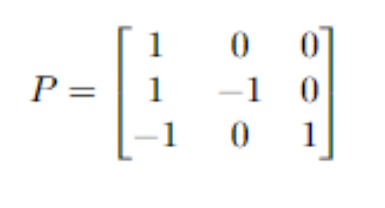
• In the P matrix, the rows are the views and the columns are the stocks. So we have three views and three stocks, hence the dimension is 3x3. Let’s consider row 2 for the view rA>rB by 2%. As stock A is bullish, it is assigned +1 and rB is bearish, it is assigned -1. This is a relative view. The first row is an absolute view, here we have information about rA only, hence +1 at the first column. Also, you can observe that for relative views, the sum of the row is 0.
• But some of the papers also have argued that assigning 1 and -1 is not a good heuristic. Hence, we should assign the relative market cap weights. For example, if the market cap of A is $2 Billion and B is $ 3 billion, then the relative weights are 0.4 and -0.6.
• Now, we will check the Q or the views vector. Again, the views are rA will be up by 5%, rA>rB by 2%, and rc>rA by 0.5%.

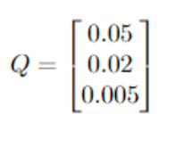
• It is #Views x 1 matrix, where are just quantifying our views. As mentioned earlier, our views have some uncertainty attached to them in form of ϵ. For each view, we have some uncertainty and it is normally distributed (assumption) as N(0, Ω).

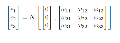
• In the B&L model, the uncertainty Ω can be calculated as Ω = τPSP`. The S matrix is the variance-covariance matrix in our utility function. Here τ is a scalar which is an empirical value equal to 0.025 (as per the paper) or sometimes is taken as 1. You can also provide confidence or uncertainty about your views. If you are not providing, then the above formula will compute the uncertainty of your views with respect to the market.
• So Ω represents the uncertainty in our views, and inv(Ω) measures the confidence of our views.
• Let’s now go over all the variables and what they mean

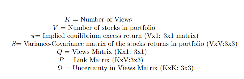
• Vx1 means the number of rows is proportional to the number of views. We have also written the dimension of each matrix based on our current example after the semicolon.
• We know that Ω = τPSP`, and the confidence in views is just the inverse of the Ω. The Black and Litterman model is just the weighted average of two things: π or implied equilibrium excess return like S&P500 return or any benchmark return that you will choose AND our views. If the uncertainty in our views is high, then we will assign more weight to π and lower weight to Q, and vice versa.
• So the excess return estimate of our portfolio is given by

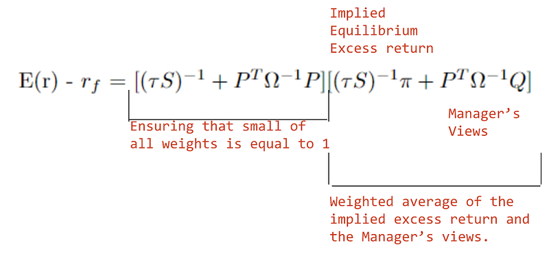
• The first term in the B&L model is kind of normalizing the weights given to each of the implied excess return and views return so that they will sum to 1. Now, the posterior covariance is given by

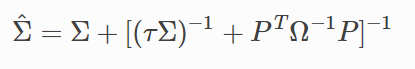
• The inversion of Ω matrix is sometimes computationally infeasible because it might be invertible. Hence sometimes, the posterior return and variance-covariance matrix is written as

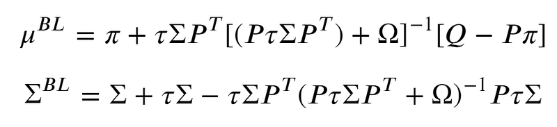
• Now after getting the weights, you can compute the weights of the portfolio from the MSR (Maximum Sharpe ratio) portfolio or the tangency portfolio.

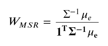
• Here the μ and ∑ are the posterior returns and covariance matrices from the B&L model. The denominator ensures that the sum of the weights is equal to 1.
• This diagram explains it really well

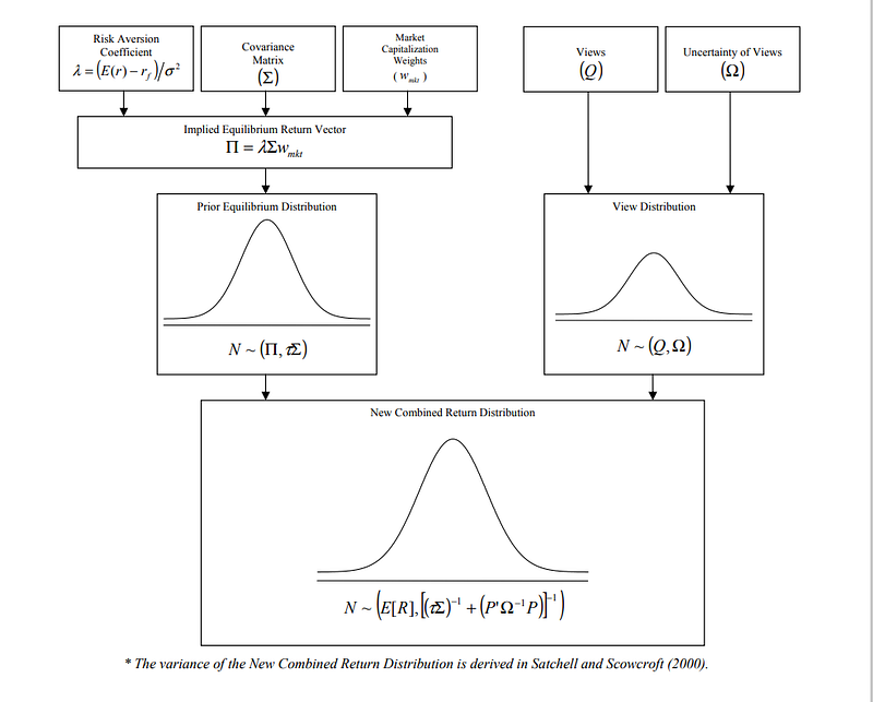
This brings us to the end of the specialization and we have covered all the modules in Course 1 and Course 2. All the articles can be found here. If you have queries or suggestions, then I am one comment away.