Making Sense of Big Data

BigQuery Hack: Flexible Queries For Any Number of Columns

How can we use BigQuery to handle tables with many columns? Here’s a how using scripting and table metadata.

BigQuery (BQ) is a Petabyte-ready proprietary Google data warehouse product. Pretty much every day in my work, I use BQ to process billions of rows of data. But sometimes, tricky situations arise. For example, what if my table has a large number of rows and columns? How does BQ deal with that?

As with all other SQL languages, besides a few syntactical tricks such as * and EXCEPT, every query requires us to manually enter the names of all the desired columns. But what if I have a table with hundreds of columns, and I want to compute, say, all the pair-wise correlations? Using the CORR function, wouldn’t I need to manually enter 100 ✕ 100 ~ 10,000/2 combinations?

Of course, I could leverage BASH/python to grab the column names and run some special scripts to get the job done. But wouldn’t it be great if we can avoid setting up different connectors and do everything natively in BQ?

Well thanks to BQ’s scripting capability and table metadata, it turns out that this is possible after all! So, let’s dive into some test data and see how it works.

Data Sample

Let’s grab some sample data. We’ll use BQ’s public dataset on Chicago taxi trips. Here’s the query to create our own table in our own dataset (MyDataSet):

Note that we added a partition column using PARTITION BY, which is always a good idea. The query will cost 13GB = $0.065. If we want to minimize cost even further, we can instead use CREATE VIEW instead (preview won’t be available though).

The final table should look like this:

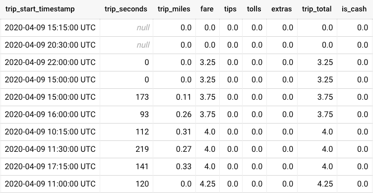
The goal here is to compute the pair-wise correlations between all of the variables (trip_seconds, trip_miles, fare, … , is_cash ). How do we proceed?

Columns to Rows

How do we query all the columns without explicitly referencing all the columns? Well, we can find a way to restructure the data such that multiple columns become a single row. How to do that? We can use ARRAY and STRUCT to create a sort of mock dictionary in BQ, effectively transposing columns into rows. This is what the end result would look like:

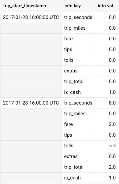
How do we create this structure? Here’s the query:

Note that we used [] and STRUCT to explicitly create the arrays. Of course, the query is still referring to the names of individual columns, which can quickly become unwieldy when the column numbers are too large. To solve this issue, we can:

1. Query INFORMATION_SCHEMA.COLUMNS to get all the relevant columns
2. Use FORMAT to construct a query string using the column information
3. Use EXECUTE IMMEDIATE to execute the constructed query string

All these steps can be strung together in a BQ script. Let’s break this down step-by-step.

BQ Scripting Using Metadata

We can get all the table metadata in a given dataset using various metadata tables. For column-related information, we can simply query

SELECT * FROM MyDataSet.INFORMATION_SCHEMA.COLUMNS

(The query is free since it processes 0 bytes)

For instance, we can extract all the numeric columns:

To extract all the numeric columns, we applied a filter on data_type. There are other possibilities using ordinal_position and/or is_partition_column.

Now, we don’t just want the column names; we want to construct a query string for the EXECUTE IMMEDIATE command. So we use BQ scripting, and convert the column names into an array of strings that can facilitate our query string construction later:

We used FORMAT to convert column_name into the 'STRUCT(... key, ... val)' pattern we used earlier for transposing columns into rows.

ARRAY converts the result of the query into an array, which gets stored into the variable query_ary for use inside a BQ script (marked by BEGIN ... END).

Now we are ready to construct our column transposition query, but without making reference to any specific column names!

We added two extra steps:

1. Format the array of strings query_ary into a query string query_string
2. Use EXECUTE IMMEDIATE to execute the constructed query.

Note that there isn’t a single mention of any of the columns in our BQ script!

Pair-wise Correlation

We are still missing a final step: How do we compute pair-wise correlations using our transposed table? This can be done using a simple aggregation (which can be inserted into our BQ script above):

The query does the following:

1. UNNEST the info array twice, creating all possible combinations of items in the array
2. i1 < i2 removes duplicates, and ensures that only combinations comparing different variables are kept
3. GROUP BY and CORR compute the correlation for each unique pair, using FORMAT to construct a nice-looking output

The end result should look like this:

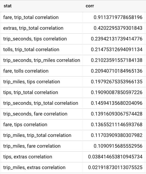
Not surprisingly, the largest correlation comes from trip_total and fare, as trip_total is equal to fare + tips + tolls + extras and the taxi fare is likely the largest contribution to the total cost of a ride. More surprisingly, trip_miles and trip_seconds aren’t all that strongly correlated with trip_total, indicating that longer trips don’t necessarily lead to a significant income boost for the driver.

We can also look at the most negative correlations:

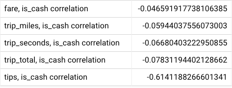
Interestingly, cash payment seems to correlate to a reduction in tips! One might think that this is because cash is likely used to pay for cheaper trips, but that correlation isn’t so strong. Another possibility may be that the cash tips are not reported all the time, or that cash usage is associated with less affluent (non-business) passengers, but these are of course speculations.

Conclusion

Using BQ scripting and table metadata, we can scale analytics in BQ both vertically (large number of rows) and horizontally (large number of columns).

If you found this article helpful, you may also be interested in my other BQ hacks. Feel free to leave a comment/question, and happy BQ hacking! 👋