Tackling Bias-Variance Problems | Towards AI

Bias-Variance Tradeoff Illustration Using Pylab

In statistics and machine learning, the bias-variance tradeoff is the property of a set of predictive models whereby models with a lower bias in parameter estimation have a higher variance of the parameter estimates across samples and vice versa. The bias-variance dilemma or problem is the conflict in trying to simultaneously minimize these two sources of error that prevent supervised learning algorithms from generalizing beyond their training set:

• The bias is an error from erroneous assumptions in the learning algorithm. High bias can cause an algorithm to miss the relevant relations between features and target outputs (underfitting).
• The variance is an error from sensitivity to small fluctuations in the training set. High variance can cause an algorithm to model the random noise in the training data, rather than the intended outputs (overfitting).

In this article, we illustrate the bias-variance problem using PyLab. Using an example, we discuss the concepts of underfitting (bias error) and overfitting (variance error).

Example: Position of an Object Hurled Upwards into the Air

We consider an experiment in which an object has been hurled into the air and its position measured as a function of time. The data obtained from this hypothetical experiment are shown below:

#import necessary libraries
import pylab
import numpy as np
import matplotlib.pyplot as plt

#create the dataset
t = np.linspace(0,1,11)
h = np.array([1.67203, 1.79792, 2.37791,2.66408,2.11245, 2.43969,1.88843, 1.59447,1.79634,1.07810,0.21066])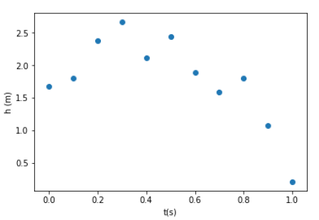

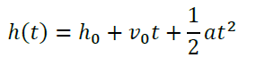
From our studies of mechanics, we know that the height should vary as the square of the time, so instead of a linear fit to the data we should use a quadratic one:

To illustrate the bias-variance problem, let's return to the position data and fit a linear, a quadratic, and a degree = 10 polynomial to the data:

plt.figure(figsize=(15,5))

# fig 1
plt.subplot(131)
#perform linear fit using pylab
degree = 1
model=pylab.polyfit(t,h,degree)
est_h=pylab.polyval(model,t)

#calculating R-squared value
R2 = 1 - ((h-est_h)**2).sum()/((h-h.mean())**2).sum()

#plot of observed and modeled data
pylab.scatter(t,h, c='b', label='observed')
pylab.plot(t,est_h, c='r', label='predicted:' + ' R2' '='+ ' ' + str(round(R2,4)))
pylab.xlabel('t(s)')
pylab.ylabel('h(m)')
pylab.title('linear model is not good (underfit)')
pylab.legend()

# fig 2
plt.subplot(132)
#perform quadratic fit using pylab
degree = 2
model=pylab.polyfit(t,h,degree)
est_h=pylab.polyval(model,t)

#calculating R-squared value
R2 = 1 - ((h-est_h)**2).sum()/((h-h.mean())**2).sum()

#plot of observed and modeled data
pylab.scatter(t,h, c='b', label='observed')
pylab.plot(t,est_h, c='r', label='predicted:' + ' R2' '='+ ' ' + str(round(R2,4)))
pylab.xlabel('t(s)')
pylab.ylabel('h(m)')
pylab.title('quadratic model is what we need')
pylab.legend()

# fig 3
plt.subplot(133)
#perform higher-degree fit using pylab
degree = 10
model=pylab.polyfit(t,h,degree)
est_h=pylab.polyval(model,t)

#calculating R-squared value
R2 = 1 - ((h-est_h)**2).sum()/((h-h.mean())**2).sum()

#plot of observed and modeled data
pylab.scatter(t,h, c='b', label='observed')
pylab.plot(t,est_h, c='r', label='predicted:' + ' R2' '='+ ' ' + str(round(R2,4)))
pylab.xlabel('t(s)')
pylab.ylabel('h(m)')
pylab.title('degree=10 captures random error (overfit)')
pylab.legend()

pylab.show()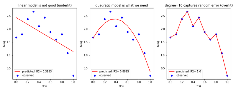

For the linear fit, the R2 (R-Squared) parameter is 0.3953 which is pretty low. If we had a good fit, we would expect the R2 value to be closer to 1.0. For the quadratic fit, the R2 value is 0.8895. The quadratic fit is thus a considerable improvement over the linear one. Using a degree = 10 polynomial, we find an R2 value which is equal to 1.0. We see that the higher degree polynomial is capturing both real and random effects. In this problem, our knowledge of mechanics dictates that there is no advantage in going to higher-order approximations beyond the quadratic model.

In summary, we’ve discussed the bias-variance problem using a very simple example. We’ve seen that the primary factor in determining a good fit is the validity of the functional form to which you’re fitting. Certainly, theoretical or analytic information about the physical problem should be incorporated into the model whenever it’s available. Generally, a simple model with fewer model parameters is always easier to interpret compared to an overly complex model.

References

1. Bias-variance tradeoff on Wikipedia.
2. A First Course in Computational Physics by Paul L. DeVries, John Wiley & Sons, 1994.